Una introducción práctica a SDMX y a la automatización de la extracción de datos de organismos internacionales
Esta es una entrada que quería escribir hace algún tiempo y que había prometido en otro post similar hace algunas semanas.
Cuando uno comienza a realizar análisis macroeconómicos -tanto para análisis como para presentaciones- el flujo de trabajo usual implica ir a la fuente de información -usualmente algún organismo internacional que agrega la información-, descargarse el conjunto de datos y luego importarlo en la herramienta de preferencia para proceder con el análisis.
Este flujo de trabajo, sin embargo, tiene bastantes inconvenientes. En primer lugar, no es replicable: existen varios pasos manuales que no quedan estrictamente documentados. Además, no es escalable, ya que si hubiese alguna nueva variable necesaria para el análisis y no tomada en cuenta en la primera extracción de datos el proceso debe repetirse nuevamente desde el inicio.
Por tanto, para el analista aplicado, se hace imprescindible automatizar el proceso de extracción de datos, de tal manera que la mayor parte del trabajo esté centrada en el análisis y menos en la plomería para contar con la información necesaria.
En este sentido, lo óptimo es contar con una API (del inglés, application programming interfase) que permita encontrar, entender y extraer la información rápidamente, de tal manera que el análisis sea totalmente reproducible y escalable. Por ejemplo, en entradas anteriores mostré cómo, de manera simplificada, acceder a la API de la CEPAL y a la del World Economic Outlook que publica el Fondo Monetario Internacional (FMI) para automatizar el flujo.
En esta entrada, sin embargo, quiero expandir las fuentes de información y ofrecer, al menos conceptualmente, un método general que permita acceder a información de organismos internacionales de forma sistemática. Esto es posible gracias a un modelo de información o protocolo estandarizado denominado SDMX y que permite acceder a los datos de forma más o menos homogénea.
En lo que sigue de esta entrada se revisará conceptualmente el modelo SDMX, se mostrará un flujo relativamente simplificado para extraer información y se mostrarán algunos ejemplos aplicados. Finalmente, para el caso del FMI, se ha creado una librería denominda imfapi que facilita la extracción de datos en base a la API SDMX que tiene actualmente el FMI y que se explora a continuación.
Qué es SDMX
Como se indica en su página web oficial:
SDMX, que significa Statistical Data and Metadata eXchange (Intercambio de Datos y Metadatos Estadísticos), es un estándar ISO diseñado para describir datos y metadatos estadísticos, normalizar su intercambio y mejorar su distribución eficiente entre organizaciones estadísticas y similares.
SDMX está patrocinado por ocho organizaciones internacionales:
- Banco de Pagos Internacionales (BIS),
- Banco Central Europeo (BCE),
- Oficina Estadística de la Unión Europea (Eurostat),
- Organización Internacional del Trabajo (OIT),
- Fondo Monetario Internacional (FMI),
- Organización para la Cooperación y el Desarrollo Económicos (OCDE),
- División de Estadística de las Naciones Unidas (UNSD) y
- Banco Mundial (WB)
Cada una de estas organizaciones ha implementado SDMX en sus sistemas de información estadística y provee APIs con esta estructura para su consulta. Esto se puede ver en la tabla a continuación:
| ORG | API SDMX | Documentación |
|---|---|---|
| BIS | https://stats.bis.org/api/v1 | BIS SDMX Tech Spec |
| BCE | https://data-api.ecb.europa.eu/service | ECB API Overview |
| Eurostat | https://ec.europa.eu/eurostat/api/dissemination | Eurostat API |
| OIT | https://sdmx.ilo.org/rest | ILOSTAT SDMX User Guide |
| FMI | https://sdmxcentral.imf.org/sdmx/v2/ | IMF Data APIs |
| OCDE | https://sdmx.oecd.org/public/rest/ | OECD Data API Explainer |
| UNSD | http://data.un.org/WS/rest/ | UN SDMX / SDG API Manual |
| WB | https://api.worldbank.org/v2/sdmx/rest/ | World Bank SDMX API Queries |
Así, el analista puede acceder a una amplia gama de datos macroeconómicos y sociales de diversas fuentes internacionales utilizando un enfoque estandarizado.
Flujo de trabajo general para extraer datos SDMX
Aunque cada API puede tener sus particularidades y el modelo SDMX es bastante amplio, el flujo de trabajo general para extraer datos utilizando APIs SDMX puede resumirse en cuatro pasos. Cada uno corresponde a un concepto clave dentro de la arquitectura SDMX y permite entender cómo están organizados y expuestos los datos por los organismos estadísticos.
- Identificación del dataflow. El primer paso consiste en identificar el dataflow. Un dataflow es, conceptualmente, el contenedor de un conjunto de datos temático. Funciona como la “base de datos” o el dominio estadístico que publica una institución (por ejemplo, estadísticas monetarias, balances bancarios, tipos de cambio o indicadores macroeconómicos). Identificar el dataflow adecuado implica revisar la lista de dataflows disponibles en la API y seleccionar aquel que contiene la información relevante para el análisis que se desea realizar. Sin este paso, no es posible avanzar hacia una consulta válida, ya que todo dataset SDMX parte de un dataflow específico.
- Obtención de la estructura de datos. Una vez seleccionado el dataflow, el siguiente paso es obtener la estructura de datos asociada, conocida como Data Structure Definition (DSD). Conceptualmente, la DSD es el esquema lógico del conjunto de datos: describe cómo están organizadas las observaciones y qué elementos intervienen en su identificación. La DSD especifica las dimensiones (como país, indicador, frecuencia o moneda), que son variables clave que clasifican los datos y determinan cómo se combinan para formar series u observaciones. También define la medida principal, que es el valor numérico del dato (por ejemplo, el índice de precios o un saldo monetario), así como los atributos adicionales que proporcionan información contextual (como la unidad, el método de ajuste estacional o el estatus de la observación). Entender esta estructura es esencial para saber qué filtros se pueden aplicar y cómo debe construirse la consulta. 3.Consulta del codelist. El tercer paso consiste en consultar las codelists. Cada dimensión definida en la DSD tiene asociada un codelist, que es el conjunto autorizado de valores posibles para esa dimensión. Las codelists funcionan como un diccionario estándar de códigos que permiten garantizar la interoperabilidad entre instituciones y sistemas. Por ejemplo, una codelist puede contener todos los códigos de países, los tipos de frecuencia temporal (anual, trimestral, mensual), o los distintos indicadores dentro de un dominio estadístico. Consultarlas es fundamental para saber qué valores se pueden usar al filtrar una consulta y cómo deben codificarse correctamente dentro de la URL o del cuerpo de la petición. Como se verá más adelante, muchas veces los codelists muestran lo posible pero no lo que es válido para un dataflow determinado. Por tanto, se tendrá que investigar si el DSD contiene restricciones en los valores y, si no, se obtendrán por fuerza bruta descargando una muestra de los datos y extrayendo los valores únicos. En cualquier caso, lo importante es que el usuario esté familiarizado con los datos.
- Extracción de datos. Finalmente, el cuarto paso es extraer los datos. Una vez que se conoce el dataflow, su estructura y los códigos permitidos para cada dimensión, es posible construir una consulta válida a la API SDMX. Esto implica seleccionar las combinaciones de códigos relevantes (por ejemplo, país, indicador y frecuencia) y aplicar filtros temporales o de detalle según lo permita la API. La respuesta suele recibirse en un formato estandarizado, como SDMX-JSON o SDMX-XML, que posteriormente puede procesarse en herramientas como
RoPythonpara análisis, visualización o integración en un pipeline reproducible. Este paso materializa todo el trabajo previo, ya que convierte la comprensión conceptual de la estructura SDMX en una solicitud concreta de datos.
Algunos ejemplos
En esta sección se realizará un ejemplo con las APIs del FMI y, posteriormente, con las APIs del Banco Central Europeo (BCE). Aunque se explicará paso a paso, se debe tener en mente que lo que vamos a hacer es:
- Identificar los dataflows disponibles (“base de datos”)
- Obtener la estructura de datos del dataflow de interés (“las variables”)
- Consultar las codelists asociadas a las dimensiones de interés (“los códigos válidos”)
- Extraer los datos (“la consulta final”)
SDMX en el FMI
El FMI tiene una colección de APIs SDMX 3.0 bastante completa que permite acceder a una amplia gama de datos macroeconómicos. Estas pueden encontrarse, luego de registrarse, aquí:
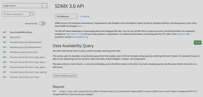
Las APIs SDMX del FMI —y en realidad cualquier API SDMX 3.0— están diseñadas siguiendo una estructura jerárquica, donde la URL funciona como un camino que va de lo más general a lo más específico. Esto permite que un usuario explore de forma progresiva el sistema estadístico, empezando por los catálogos completos y avanzando hacia un dataset concreto o incluso una sola serie temporal.
La idea fundamental es que cada segmento de la ruta añade una restricción, un filtro, o un nivel de precisión. Así, una llamada puede significar “mostrar todo”, o “dame exactamente esta estructura de datos”, dependiendo de cuántos parámetros se incluyan. Vamos a verlo por partes.
Datos disponibles: el dataflow
En primer lugar, el punto de partida es la URL base que, en este caso, es https://api.imf.org/external/sdmx/3.0. A partir de este punto podemos decir que la API del FMI se divide en dos grandes familias: una de estructura y otra de datos. La primera permite explorar los catálogos y estructuras, mientras que la segunda permite extraer datos concretos.
Por ejemplo, si a la URL base le añadimos /structure/dataflow, obtenemos el catálogo completo de dataflows disponibles en la API, es decir, estamos pidiendo “dame todos los dataflows que tiene el FMI”. Si, por otro lado, añadimos /structure/datastructure básicamente le estamos pidiendo “dame todas las DSD que tiene el FMI”. Este nivel es más bien bastante general, pues no aplica ningún filtro a la extracción, lo que es útil cuando no sabemos qué es lo que necesitamos.
Para ilustrar esto vamos a realizar el primer paso del flujo de trabajo: obtener todos los dataflows disponibles en la API del FMI y localizar el dataflow correspondiente al World Economic Outlook (WEO). Esto se puede hacer con el siguiente código en R:
# 1. Base URL SDMX 3.0 del FMI
base_url <- "https://api.imf.org/external/sdmx/3.0"


# 2. Obtener todos los dataflows
flows_resp <- httr2::request(paste0(base_url, "/structure/dataflow")) |>
  httr2::req_perform()

flows_json <- flows_resp |>
  httr2::resp_body_string() |>
  jsonlite::fromJSON(flatten = TRUE)

flows <- flows_json$data$dataflows

# Tabla de dataflows en formato tibble
df_flows <- tibble::tibble(
  id      = flows$id,
  name    = flows$names.en,
  version = flows$version,
  agency  = flows$agencyID,
  dsd_urn = flows$structure
)

df_flows |>
  dplyr::select(id, name, version, agency) |>
  dplyr::arrange(id) |>
  kableExtra::kable()
| id | name | version | agency |
|---|---|---|---|
| AFRREO | Sub-Saharan Africa Regional Economic Outlook (AFRREO) | 6.0.1 | IMF.AFR |
| ANEA | National Economic Accounts (NEA), Annual Data | 6.0.1 | IMF.STA |
| APDREO | Asia and Pacific Regional Economic Outlook (APDREO) | 6.0.0 | IMF.APD |
| BOP | Balance of Payments (BOP) | 21.0.0 | IMF.STA |
| BOP_AGG | Balance of Payments and International Investment Position Statistics (BOP/IIP), World and Country Group Aggregates | 9.0.1 | IMF.STA |
| COFER | Currency Composition of Official Foreign Exchange Reserves (COFER) | 7.0.0 | IMF.STA |
| CPI | Consumer Price Index (CPI) | 5.0.0 | IMF.STA |
| CPI_WCA | Consumer Price Index (CPI), World and Country Aggregates (CPI_WCA) | 2.0.2 | IMF.STA |
| CTOT | Commodity Terms of Trade (CTOT) | 5.0.1 | IMF.RES |
| DIP | Direct Investment Positions by Counterpart Economy (formerly CDIS) | 12.0.0 | IMF.STA |
| ED | Export Diversification (ED) | 1.0.0 | IMF.RES |
| EER | Effective Exchange Rate (EER) | 6.0.0 | IMF.STA |
| EQ | Export Quality (EQ) | 2.0.0 | IMF.RES |
| ER | Exchange Rates (ER) | 4.0.1 | IMF.STA |
| FA | Fund Accounts (FA) | 8.0.0 | IMF.STA |
| FAS | Financial Access Survey (FAS) | 4.0.0 | IMF.STA |
| FD | Fiscal Decentralization (FD) | 6.0.0 | IMF.STA |
| FDI | Financial Development Index (FDI) | 1.0.0 | IMF.MCM |
| FM | Fiscal Monitor (FM) | 5.0.0 | IMF.FAD |
| FSIBSIS | Financial Soundness Indicators (FSI), Balance Sheet, Income Statement and Memorandum Series | 18.0.0 | IMF.STA |
| FSIC | Financial Soundness Indicators (FSI), Core and Additional Indicators | 13.0.1 | IMF.STA |
| FSICDM | Financial Soundness Indicators (FSI), Concentration and Distribution Measures | 7.0.0 | IMF.STA |
| GDD | Global Debt Database (GDD) | 2.0.0 | IMF.FAD |
| GFS_BS | GFS Balance Sheet | 12.0.0 | IMF.STA |
| GFS_COFOG | GFS Government Expenditures by Function | 11.0.0 | IMF.STA |
| GFS_SFCP | GFS Stocks and Flows by Counterparty | 10.0.0 | IMF.STA |
| GFS_SOEF | GFS Statement of Other Economic Flows | 11.0.0 | IMF.STA |
| GFS_SOO | GFS Statement of Operations | 12.0.0 | IMF.STA |
| GFS_SSUC | GFS Statement of Sources and Uses of Cash | 10.0.0 | IMF.STA |
| HPD | Historical Public Debt (HPD) | 1.0.0 | IMF.FAD |
| ICSD | Investment and Capital Stock Dataset (ICSD) | 1.0.0 | IMF.FAD |
| IIP | International Investment Position (IIP) | 13.0.0 | IMF.STA |
| IIPCC | Currency Composition of the International Investment Position (IIPCC) | 13.0.0 | IMF.STA |
| IL | International Liquidity (IL) | 13.0.1 | IMF.STA |
| IMTS | International Trade in Goods (by partner country) (IMTS) | 1.0.0 | IMF.STA |
| IRFCL | International Reserves and Foreign Currency Liquidity (IRFCL) | 11.0.0 | IMF.STA |
| ISORA_2016_DATA_PUB | ISORA 2016 Data | 2.0.0 | ISORA |
| ISORA_2018_DATA_PUB | ISORA 2018 Data | 2.0.0 | ISORA |
| ISORA_LATEST_DATA_PUB | ISORA Latest Data | 4.0.0 | ISORA |
| ITG | International Trade in Goods (ITG) | 4.0.0 | IMF.STA |
| ITG_WCA | International Trade in Goods, World and Country Aggregates | 2.0.4 | IMF.STA |
| ITS | International Trade in Services (ITS) | 3.0.1 | IMF.RES |
| LS | Labor Statistics (LS) | 9.0.0 | IMF.STA |
| MCDREO | Middle East and Central Asia Regional Economic Outlook (MCDREO) | 8.0.0 | IMF.MCD |
| MFS_CBS | Monetary and Financial Statistics (MFS), Central Bank Data | 24.0.0 | IMF.STA |
| MFS_DC | Monetary and Financial Statistics (MFS), Depository Corporations | 8.0.0 | IMF.STA |
| MFS_FC | Monetary and Financial Statistics (MFS), Financial Corporations | 9.0.0 | IMF.STA |
| MFS_FMP | Monetary and Financial Statistics (MFS): Financial Market Prices | 3.0.0 | IMF.STA |
| MFS_IR | Monetary and Financial Statistics (MFS), Interest Rate | 8.0.1 | IMF.STA |
| MFS_MA | Monetary and Financial Statistics (MFS), Monetary Aggregates | 10.0.1 | IMF.STA |
| MFS_NSRF | Monetary and Financial Statistics (MFS), Non-Standard Data | 1.0.3 | IMF.STA |
| MFS_ODC | Monetary and Financial Statistics (MFS), Other Depository Corporations | 10.0.0 | IMF.STA |
| MFS_OFC | Monetary and Financial Statistics (MFS), Other Financial Corporations | 7.0.0 | IMF.STA |
| MPFT | Monetary Policy Frameworks Toolkit (MPFT) | 7.0.1 | IMF.RES |
| NSDP | National Summary Data Page (NSDP) | 7.0.0 | IMF.STA |
| PCPS | Primary Commodity Price System (PCPS) | 9.0.0 | IMF.RES |
| PI | Production Indexes (PI) | 2.0.0 | IMF.STA |
| PIP | Portfolio Investment Positions by Counterpart Economy (formerly CPIS) | 4.0.0 | IMF.STA |
| PI_WCA | Production Indexes, World and Country Group Aggregates | 1.0.0 | IMF.STA |
| PPI | Producer Price Index (PPI) | 3.0.0 | IMF.STA |
| PSBS | Public Sector Balance Sheet (PSBS) | 2.0.0 | IMF.FAD |
| QGDP_WCA | Quarterly Gross Domestic Product (GDP), World and Country Aggregates | 3.0.0 | IMF.STA |
| QGFS | Quarterly Government Finance Statistics (QGFS) | 12.0.0 | IMF.STA |
| QNEA | National Economic Accounts (NEA), Quarterly Data | 7.0.0 | IMF.STA |
| SDG | IMF Reported SDG Data | 2.0.1 | IMF.STA |
| SPE | Special Purpose Entities (SPEs) | 13.0.0 | IMF.STA |
| SRD | Structural Reform Database (SRD) | 1.0.0 | IMF.RES |
| TAXFIT | Tax and Benefits Analysis Tool (TAXFIT) | 2.0.3 | IMF.RES |
| TEG | Trade in Low Carbon Technology Goods (TEG) | 3.0.2 | IMF.STA |
| WEO | World Economic Outlook (WEO) | 9.0.0 | IMF.RES |
| WHDREO | Western Hemisphere Regional Economic Outlook (WHDREO) | 5.0.0 | IMF.WHD |
| WPCPER | Crypto-based Parallel Exchange Rates (Working Paper dataset WP-CPER) | 6.0.0 | IMF.STA |
En la tabla anterior podemos ver todos los dataflows disponibles en la API del FMI. Cada dataflow tiene un identificador único (id), un nombre descriptivo (name), una versión (version), una agencia responsable (agency) y un URN (del inglés, Uniform Resource Name) que no se reproduce por motivos de espacio pero que apunta a su estructura de datos asociada (dsd_urn).
En nuestro caso nos interesa el dataflow WEO. Podemos filtrar el dataflow de interés de la siguiente manera:
# Nos quedamos con el dataflow WEO
weo <- df_flows |>
  dplyr::filter(id == "WEO")

weo |>
  kableExtra::kable()
| id | name | version | agency | dsd_urn |
|---|---|---|---|---|
| WEO | World Economic Outlook (WEO) | 9.0.0 | IMF.RES | urn:sdmx:org.sdmx.infomodel.datastructure.DataStructure=IMF.RES:DSD_WEO(9.0+.0) |
Estructura de datos: las dimensiones
Ahora que tenemos el dataflow de interés, el siguiente paso es entender qué varialbles (dimensions) están disponibles en su estructura de datos. Para ello, el API que debemos consultar tiene la forma de: /structure/datastructure/{agency}/{dsd_id}/{version}, donde {agency}, {dsd_id} y {version} son los componentes que debemos extraer del URN del dataflow WEO. Nótese que, en el caso de no indicar estos tres campos se corre el riesgo de obtener información desactualizada.
¿Cómo obtenemos esta información? Lo bueno es que, al momento de consultar el dataflow esta información se provee en el URN asociada:
# Parsear el URN del datastructure de WEO
urn <- weo$dsd_urn
urn
## [1] "urn:sdmx:org.sdmx.infomodel.datastructure.DataStructure=IMF.RES:DSD_WEO(9.0+.0)"
Nótese que aquí tenemos las 3 piezas esenciales:
- La agencia responsable del DSD:
IMF.RES - El identificador del DSD:
DSD_WEO - La versión del DSD:
9.0+.0
Para extraer estas piezas de forma sistemática podemos usar expresiones regulares en R de la siguiente manera:
m     <- base::regexec("DataStructure=([^:]+):([^()]+)\\(([^)]+)\\)", urn)
parts <- base::regmatches(urn, m)[[1]]

agency_dsd  <- parts[2]   # p.ej. "IMF.RES"
dsd_id      <- parts[3]   # p.ej. "DSD_WEO"
version_dsd <- parts[4]   # p.ej. "9.0+.0"


# Descargar el datastructure de WEO y ver dimensiones

dsd_url <- paste0(
  base_url,
  "/structure/datastructure/",
  agency_dsd, "/", dsd_id, "/", version_dsd
)
dsd_url
## [1] "https://api.imf.org/external/sdmx/3.0/structure/datastructure/IMF.RES/DSD_WEO/9.0+.0"
Ahora que tenemos la URL del datastructure de WEO, podemos descargarlo y ver las dimensiones disponibles:
dsd_resp <- httr2::request(dsd_url) |>
  httr2::req_perform()

dsd_json <- dsd_resp |>
  httr2::resp_body_string() |>
  jsonlite::fromJSON(flatten = TRUE)

# Dimensiones "normales": COUNTRY, INDICATOR, FREQUENCY
dims_main <- dsd_json$data$dataStructures$dataStructureComponents.dimensionList.dimensions[[1]] |>
  tibble::as_tibble() |>
  dplyr::select(position, id, type)

# Dimensión de tiempo: TIME_PERIOD
time_dim <- dsd_json$data$dataStructures$dataStructureComponents.dimensionList.timeDimensions[[1]] |>
  tibble::as_tibble() |>
  dplyr::select(position, id, type)

# Orden completo de dimensiones
dims_clean <- dplyr::bind_rows(dims_main, time_dim) |>
  dplyr::arrange(position)

dims_clean |>
  kableExtra::kable()
| position | id | type |
|---|---|---|
| 0 | COUNTRY | Dimension |
| 1 | INDICATOR | Dimension |
| 2 | FREQUENCY | Dimension |
| 3 | TIME_PERIOD | TimeDimension |
En la tabla anterior podemos ver las dimensiones disponibles en el dataflow WEO (COUNTRY, INDICATOR, FREQUENCY y TIME_PERIOD). Estas dimensiones son esenciales para entender cómo se organizan los datos y qué filtros podemos aplicar al momento de extraer información específica.
Nótese también que, aunque la consulta se ha obtenido sin errores, previamente se exploró dsd_json para entender dónde y cómo estaba almacenando la información.
Codelists: los códigos válidos
Como tercer paso, y antes de extraer los datos, es importante conocer los códigos válidos para cada dimensión del dataset. Esto es fundamental porque, al construir la consulta final, debemos asegurarnos de usar los valores exactos que la API reconoce. Caso contrario nos devolverá un error. Por ejemplo, si queremos obtener el crecimiento del PIB real para un país específico, necesitamos saber cómo codifica el FMI el país, el indicador y la frecuencia. No basta con escribir “Bolivia” o “Real GDP growth”: hay que usar los códigos oficiales definidos por la estructura del dataset.
Cada una de las dimensiones del WEO —COUNTRY, INDICATOR, FREQUENCY y TIME_PERIOD— tiene un conjunto autorizado de valores posibles: el codelist. Por ejemplo, los códigos de país pueden ser BOL, ARG o USA; los indicadores pueden ser NGDP_RPCH, LUR u otros; y las frecuencias válidas suelen ser A (anual), Q (trimestral), etc. Un detalle importante es que cada dataset puede tener codelists distintos, aun para conceptos relativamente similares. El FMI podría usar una lista de países para WEO, otra para BOP (Balance of Payments), y otra para estadísticas monetarias. Esto significa que no necesariamente los códigos que funcionan para un dataflow van a funcionar para otro.
Por eso, si queremos consultar datos del WEO, no podemos inventarnos los códigos ni confiar en listas antiguas: se debe consultar directamente al FMI las codelists oficiales asociadas. La única manera segura de hacerlo es comenzar por el dataflow, obtener su estructura (la DSD) y, desde allí, recuperar las listas de códigos correctas para cada dimensión. Este procedimiento asegura que la consulta sea reproducible, exacta y totalmente compatible con la definición que el FMI usa internamente.
Para obtener estas codelists asociadas al dataflow WEO, utilizamos una URL específica de la API SDMX del FMI. El patrón general es: /structure/dataflow/{agency}/{dataflow_id}/+, donde {agency} y {dataflow_id} provienen del propio dataflow (en nuestro caso, IMF.RES y WEO, respectivamente). El símbolo + indica que queremos la versión más reciente disponible. Pero lo realmente importante son los parámetros que añadimos al final: ?detail=full&references=descendants1.
Para nuestro caso, la URL completa para obtener las codelists del WEO es la siguiente:
weo_struct_url <- paste0(
  base_url,
  "/structure/dataflow/",
  weo$agency, "/", weo$id, "/+",
  "?detail=full&references=descendants"
)
weo_struct_url
## [1] "https://api.imf.org/external/sdmx/3.0/structure/dataflow/IMF.RES/WEO/+?detail=full&references=descendants"
Al realizar la petición a esta URL, obtenemos una respuesta que incluye todas las codelists asociadas al dataflow WEO. Podemos procesar esta respuesta para extraer las codelists específicas que necesitamos para cada dimensión:
weo_struct_resp <- httr2::request(weo_struct_url) |>
  httr2::req_perform()

weo_struct_json <- weo_struct_resp |>
  httr2::resp_body_string() |>
  jsonlite::fromJSON(flatten = TRUE)

# Tabla de codelists
codelists_tbl <- weo_struct_json$data$codelists

codelists_tbl |>
  dplyr::select(id, name, version, agencyID) |>
  head() |>
  kableExtra::kable()
| id | name | version | agencyID |
|---|---|---|---|
| CL_DERIVATION_TYPE | Derivation Type | 1.2.1 | IMF |
| CL_VALUATION | Valuation | 2.4.0 | IMF |
| CL_GFS_STO | GFS Stocks, Transactions, Other Flows | 2.9.0 | IMF |
| CL_ACCOUNTING_ENTRY | Accounting Entry | 2.2.1 | IMF |
| CL_UNIT | Unit of Measure | 2.11.0 | IMF |
| CL_ACCESS_SHARING_LEVEL | Access and Sharing Level | 1.0.2 | IMF |
Nótese que en la tabla anterior se ha extraído bastante información sobre las codelists disponibles para el dataflow WEO. En el código a continuación vamos a resumir un poco lo extraído:
# Vista resumida de las codelists
weo_codelists_overview <- tibble::tibble(
  cl_id   = codelists_tbl$id,
  cl_name = ifelse(is.na(codelists_tbl$names.en),
                   yes = codelists_tbl$name,
                   no = codelists_tbl$names.en
                   ),
  n_codes = sapply(codelists_tbl$codes, nrow)
)

weo_codelists_overview |>
  dplyr::arrange(desc(cl_id)) |>
  kableExtra::kable()
| cl_id | cl_name | n_codes |
|---|---|---|
| CL_WEO_INDICATOR | World Economic Outlook (WEO) Indicator | 145 |
| CL_WEO_COUNTRY | World Economic Outlook (WEO) Country | 338 |
| CL_VALUATION | Valuation | 26 |
| CL_UNIT_MULT | Unit Multiplier | 31 |
| CL_UNIT | Unit of Measure | 270 |
| CL_TRANSFORMATION | Transformation | 487 |
| CL_TRADE_FLOW | Trade flow | 50 |
| CL_TOPIC | Topic | 118 |
| CL_S_ADJUSTMENT | Seasonal Adjustment | 17 |
| CL_STATISTICAL_MEASURES | Statistical Measures | 23 |
| CL_SOC_CONCEPTS | Social Concepts | 31 |
| CL_SEX | Sex | 9 |
| CL_SEC_CLASSIFICATION | Security Classification | 6 |
| CL_SECTOR | Institutional Sector | 288 |
| CL_REPORTING_PERIOD_TYPE | REPORTING_PERIOD_TYPE | 6 |
| CL_PRICES | Prices | 15 |
| CL_OVERLAP | IMF Data Overlap | 1 |
| CL_ORGANIZATION | Organization | 1588 |
| CL_OBS_STATUS | Observation Status | 22 |
| CL_NA_STO | NA Stocks, Transactions, Other Flows | 636 |
| CL_MFS_INSTR | Monetary and Financial Instruments | 18 |
| CL_METHODOLOGY | Methodology | 69 |
| CL_LANGUAGE | Language | 93 |
| CL_INT_TTC | Interest Rate types, terms and conditions | 101 |
| CL_INT_ACC_ITEM | International accounts item | 507 |
| CL_INSTR_ASSET | Instrument and assets classification | 342 |
| CL_INDEX_TYPE | Index type | 49 |
| CL_GFS_STO | GFS Stocks, Transactions, Other Flows | 389 |
| CL_GENDER | Gender | 15 |
| CL_FUNCTIONAL_CAT | Functional category | 72 |
| CL_FSENTRY | Flow or stock entry | 43 |
| CL_FREQ | Frequency | 6 |
| CL_FI_MATURITY | Maturity of Financial Instrument | 32 |
| CL_EXRATE | Exchange Rate | 37 |
| CL_DERIVATION_TYPE | Derivation Type | 12 |
| CL_DEPARTMENT | Department | 34 |
| CL_DECIMALS | Decimals | 16 |
| CL_CURRENCY | Currency | 177 |
| CL_COUNTRY | Country | 337 |
| CL_CONF_STATUS | Confidentiality Status | 12 |
| CL_COMMODITY | Commodity | 135 |
| CL_COICOP_2018 | COICOP 2018 | 16 |
| CL_COICOP_1999 | COICOP 1999 | 15 |
| CL_COFOG | COFOG | 190 |
| CL_CIVIL_STATUS | Civil (or Marital) Status | 8 |
| CL_ACCOUNTS | Macroeconomic and financial accounts | 40 |
| CL_ACCOUNTING_ENTRY | Accounting Entry | 82 |
| CL_ACCESS_SHARING_LEVEL | Access and Sharing Level | 8 |
En la tabla anterior podemos ver un resumen de las codelists disponibles para el dataflow WEO. Cada codelist tiene un identificador (cl_id), un nombre descriptivo (cl_name) y el número de códigos que contiene (n_codes). En nuestro caso, nos interesan particularmente las codelists asociadas a las dimensiones COUNTRY, INDICATOR y FREQUENCY: CL_WEO_COUNTRY, CL_WEO_INDICATOR y CL_FREQUENCY.
Por ejemplo, en el caso de CL_WEO_COUNTRY:
weo_country_codes <- codelists_tbl$codes[[which(codelists_tbl$id == "CL_WEO_COUNTRY")]] |>
  tibble::as_tibble() |>
  dplyr::transmute(
    code    = id,
    name_en = names.en  # en CL_WEO_COUNTRY viene como names.en1
  )
weo_country_codes |>
  head(20) |>
  kableExtra::kable()
| code | name_en |
|---|---|
| GX123 | Other Advanced Economies (Advanced Economies excluding G7 and Euro Area countries) |
| AFG | Afghanistan, Islamic Republic of |
| ALB | Albania |
| DZA | Algeria |
| ASM | American Samoa |
| AND | Andorra, Principality of |
| AGO | Angola |
| AIA | Anguilla, United Kingdom-British Overseas Territory |
| ATG | Antigua and Barbuda |
| ARG | Argentina |
| ARM | Armenia, Republic of |
| ABW | Aruba, Kingdom of the Netherlands |
| AUS | Australia |
| AUT | Austria |
| AZE | Azerbaijan, Republic of |
| BHS | Bahamas, The |
| BHR | Bahrain, Kingdom of |
| BGD | Bangladesh |
| BRB | Barbados |
| BLR | Belarus, Republic of |
En la tabla anterior podemos ver los códigos de país válidos para el dataflow WEO. Cada país tiene un código (code) y un nombre descriptivo en inglés (name_en). Estos códigos son esenciales para construir consultas precisas al API del FMI.
Ahora, procedemos a buscar los INDICATOR disponibles en el WEO:
weo_indicator_codes <- codelists_tbl$codes[[which(codelists_tbl$id == "CL_WEO_INDICATOR")]] |>
  tibble::as_tibble() |>
  dplyr::transmute(
    code    = id,
    name_en = names.en
  )

weo_indicator_codes |>
  kableExtra::kable()
| code | name_en |
|---|---|
| LUR | Unemployment rate |
| PCOALSA | Coal, South Africa, Export price, US dollars per metric tonne |
| DSP | External debt: total debt service, amortization, US dollar |
| DSI | External debt: total debt service, interest, US dollar |
| DSP_NGDPD | External debt: total debt service, amortization, Percent of GDP |
| BX | Exports of goods and services, US dollar |
| BM | Imports of goods and services, US dollar |
| DS | External debt: total debt service, US dollar |
| TTPCH | Terms of trade of goods and services, percent change |
| DSI_NGDPD | External debt: total debt service, interest, Percent of GDP |
| NGDP_RPCHMK | Gross domestic product (GDP), Constant prices, Percent |
| NGDPD | Gross domestic product (GDP), Current prices, US dollar |
| PTEA | Tea, Kenyan, Unit prices, US cents per kilogram |
| DS_NGDPD | External debt: total debt service, Percent of GDP |
| D | External debt, US dollar |
| NGDP_D | Gross domestic product (GDP), Price deflator, Index |
| NGDP_RPCH | Gross domestic product (GDP), Constant prices, Percent change |
| TTTPCH | Terms of trade of goods, percent change |
| NGDP_R | Gross domestic product (GDP), Constant prices, Domestic currency |
| NGDP | Gross domestic product (GDP), Current prices, Domestic currency |
| NGSD_NGDP | Gross national savings, Percent of GDP |
| PSUNO | Sunflower oil, Export price, US dollars per metric tonne |
| PNGASEU | Natural gas, EU, Unit prices, US dollars per million metric British thermal units of gas |
| PZINC | Zinc, Unit prices, US dollars per metric tonne |
| PPPSH | Gross domestic product (GDP), Purchasing power parity (PPP) international dollar, percent of world GDP, Percent, ICP benchmarks 2017-2021 |
| D_NGDPD | External debt, Percent of GDP |
| PPPPC | Gross domestic product (GDP), Per capita, purchasing power parity (PPP) international dollar, ICP benchmarks 2017-2021 |
| PPPGDP | Gross domestic product (GDP), Current prices, Purchasing power parity (PPP) international dollar, ICP benchmarks 2017-2021 |
| DSP_BX | External debt: total debt service, amortization, Percent of exports of goods and services |
| PPORK | Swine, Unit prices, US cents per pound |
| PSAWMAL | Hard sawnwood, Dark Red Meranti, Unit prices, US dollars per cubic meter |
| PORANG | Orange, Import price, US dollars per metric tonne |
| PTIN | Tin, Unit prices, US dollars per metric tonne |
| PPOULT | Poultry, Unit prices, US cents per pound |
| DSI_BX | External debt: total debt service, interest, Percent of exports of goods and services |
| NGDPDPC | Gross domestic product (GDP), Current prices, Per capita, US dollar |
| PSAWORE | Soft sawnwood, Export price, US dollars per cubic meter |
| PROIL | Rapeseed oil, Unit prices, US dollars per metric tonne |
| PLAMB | Lamb, Unit prices, US cents per pound |
| PBARL | Barley, Unit prices, US dollars per metric tonne |
| PLOGORE | Soft logs, Export price, US dollars per cubic meter |
| GGR_NGDP | Revenue, General government, Percent of GDP |
| TRADEPCH | Trade of goods and services, Volume, Percent change |
| PALUM | Aluminum, Unit prices, US dollars per metric tonne |
| PLOGSK | Hard logs, import price Japan, Import price, US dollars per cubic meter |
| PWOOLC | Wool, coarse, Unit prices, US cents per kilogram |
| GGXWDN_NGDP | Net debt, General government, Percent of GDP |
| PFISH | Fishmeal, Unit prices, US dollars per metric tonne |
| NGDPRPC | Gross domestic product (GDP), Constant prices, Per capita, Domestic currency |
| PNGASJP | LNG, Asia, Unit prices, US dollars per million metric British thermal units of gas |
| LE | Employed persons, Persons for countries / Index for country groups |
| NGDPPC | Gross domestic product (GDP), Current prices, Per capita, Domestic currency |
| GGR | Revenue, General government, Domestic currency |
| PWOOLF | Wool, fine, Unit prices, US cents per kilogram |
| PCOFFOTM | Coffee, other mild Arabica, Unit prices, US cents per pound |
| PNICK | Nickel, Unit prices, US dollars per metric tonne |
| BCA | Current account balance (credit less debit), US dollar |
| PBANSOP | Bananas, Unit prices, US dollars per metric tonne |
| PRICENPQ | Rice, Thailand, Unit prices, US dollars per metric tonne |
| DS_BX | External debt: total debt service, Percent of exports of goods and services |
| PCOFFROB | Coffee, Robustas, Unit prices, US cents per pound |
| PSALM | Fish, Export price, US dollars per kilogram |
| PSUGAUSA | Sugar, No. 16, US, Import price, US cents per pound |
| GGXWDG_NGDP | Gross debt, General government, Percent of GDP |
| PCOPP | Copper, Unit prices, US dollars per metric tonne |
| PLEAD | Lead, Unit prices, US dollars per metric tonne |
| PBEEF | Beef, Import price, US cents per pound |
| BF | Financial account balance (assets less liabilities), US dollar |
| PURAN | Uranium, Unit prices, US dollars per pound |
| BCA_NGDPD | Current account balance (credit less debit), Percent of GDP |
| PHIDE | Hides, Unit prices, US cents per pound |
| PGNUTS | Groundnuts, Unit prices, US dollars per metric tonne |
| GGSB | Structural balance, General government, Domestic currency |
| BFP | Portfolio investment, Net (assets minus liabilities), US dollar |
| GGX_NGDP | Expenditure, General government, Percent of GDP |
| GGXWDG | Gross debt, General government, Domestic currency |
| GGXWDN | Net debt, General government, Domestic currency |
| NGDP_FY | Gross domestic product (GDP), Current prices, Fiscal year, Domestic currency |
| GGX | Expenditure, General government, Domestic currency |
| PRUBB | Rubber, Unit prices, US cents per pound |
| PWHEAMT | Wheat, Unit prices, US dollars per metric tonne |
| PMAIZMT | Corn, Unit prices, US dollars per metric tonne |
| GGSB_NPGDP | Structural balance, General government, Percent |
| POLVOIL | Olive oil, Unit prices, US dollars per metric tonne |
| PIORECR | Iron ore, Unit prices, US dollars per metric tonne |
| D_BX | External debt, Percent of exports of goods and services |
| BFD | Direct investment, Net (assets minus liabilities), US dollar |
| TX_RPCH | Exports of goods and services, Volume, Free on board (FOB), Percent change |
| PCOCO | Cocoa, Unit prices, US dollars per metric tonne |
| BFO | Other investment, Net (assets minus liabilities), US dollar |
| PPOIL | Palm oil, Unit prices, US dollars per metric tonne |
| NGDPRPPPPC | Gross domestic product (GDP), Constant prices, Per capita, purchasing power parity (PPP) international dollar, ICP benchmark 2021 |
| PRAWMW | Agricultural raw materials, Commodity price index |
| PSMEA | Soybean meal, Unit prices, US dollars per metric tonne |
| PCOTTIND | Cotton, Unit prices, US cents per pound |
| PCOALAU | Coal, Australia, Unit prices, US dollars per metric tonne |
| PNGASUS | Natural Gas, US Henry Hub Gas, Unit prices, US dollars per metric tonne |
| TXGM_D | Exports of manufactures, Price deflator, Free on board (FOB), Index |
| TM_RPCH | Imports of goods and services, Volume, Cost insurance freight (CIF), Percent change |
| PSOIL | Soybeans oil, Unit prices, US dollars per metric tonne |
| PSUGAISA | Sugar, No. 11, World, Unit prices, US cents per pound |
| BFF | Financial derivatives and employee stock options, Net (assets minus liabilities), US dollar |
| NGAP_NPGDP | Output gap, Percent of potential GDP |
| PSOYB | Soybeans, Unit prices, US dollars per metric tonne |
| PINDUW | Industrial materials, Commodity price index |
| GGXCNL | Net lending (+) / net borrowing (-), General government, Domestic currency |
| BFRA | Change in reserve assets, Net (assets minus liabilities), US dollar |
| TXGM_DPCH | Exports of manufactures, Price deflator, Free on board (FOB), Percent change |
| POILBRE | Brent crude, Unit prices, US dollars per barrel |
| PSHRI | Shrimp, Unit prices, US dollars per kilogram |
| GGXCNL_NGDP | Net lending (+) / net borrowing (-), General government, Percent of GDP |
| PCOALW | Coal, Commodity price index |
| PBEVEW | Beverages, Commodity price index |
| PWOOLW | Wool, Commodity price index |
| POILDUB | Dubai crude, Unit prices, US dollars per barrel |
| POILWTI | WTI crude, Unit prices, US dollars per barrel |
| PCOFFW | Coffee, Commodity price index |
| PCPI | All Items, Consumer price index (CPI), Period average |
| PSEAFW | Seafood, Commodity price index |
| PTIMBW | Timber, Commodity price index |
| GGXONLB_NGDP | Primary net lending (+) / net borrowing (-), General government, Percent of GDP |
| PSUGAW | Sugar, Commodity price index |
| POILAPSP | APSP crude oil, Unit prices, US dollars per barrel |
| PCEREW | Cereal, Commodity price index |
| PALLFNFW | All commodities, Commodity price index |
| PCPIE | All Items, Consumer price index (CPI), End-of-period (EoP) |
| GGXONLB | Primary net lending (+) / net borrowing (-), General government, Domestic currency |
| TXG_RPCH | Exports of goods, Volume, Free on board (FOB), Percent change |
| TMG_RPCH | Imports of goods, Volume, Cost insurance freight (CIF), Percent change |
| PSOFTW | Softwood, Commodity price index |
| PHARDW | Hardwood, Commodity price index |
| PCPIPCH | All Items, Consumer price index (CPI), Period average, percent change |
| PMEATW | Meat, Commodity price index |
| PFANDBW | Food and beverage, Commodity price index |
| PCPIEPCH | All Items, Consumer price index (CPI), End-of-period (EoP), percent change |
| PNFUELW | Non-fuel, Commodity price index |
| PNRGW | Energy, Commodity price index |
| LP | Population, Persons for countries / Index for country groups |
| PNGASW | Natural gas, Commodity price index |
| PPPEX | Rate, Domestic currency per international dollar in PPP terms, ICP benchmarks 2017-2021 |
| PFOODW | Food, Commodity price index |
| PMETAW | Metal, Commodity price index |
| POILAPSPW | APSP crude oil, Commodity price index |
| NID_NGDP | Gross capital formation, Percent of GDP |
| PVOILW | Vegetable oil, Commodity price index |
Finalmente, para la frecuencia:
weo_frequency_codes <- codelists_tbl$codes[[which(codelists_tbl$id =="CL_FREQ")]] |>
  tibble::as_tibble() |>
  dplyr::transmute(
    code    = id,
    name_en = names.en
  )
weo_frequency_codes |>
  kableExtra::kable()
| code | name_en |
|---|---|
| A | Annual |
| D | Daily |
| M | Monthly |
| Q | Quarterly |
| S | Half-yearly, semester |
| W | Weekly |
Una vez que tenemos los códigos válidos para las dimensiones de interés, estamos listos para proceder a la extracción de datos específicos del dataflow WEO. Este es el último paso del flujo de trabajo SDMX y nos permitirá obtener las series temporales que necesitamos para nuestro análisis macroeconómico.
Extracción de datos: la consulta final
Con los códigos válidos para las dimensiones COUNTRY, INDICATOR y FREQUENCY en mano, ya estamos en condiciones de construir la consulta final para extraer datos específicos del dataflow WEO. Desde el punto de vista de la API del FMI, el endpoint general de datos tiene la forma:
/data/{context}/{agencyID}/{resourceID}/{version}/{key}[?c]
En nuestro caso, {context} será dataflow, {agencyID} será IMF.RES, {resourceID} será WEO y {version} la última versión estable (+). Es decir, todo lo que está antes de {key} ya lo conocemos a partir de los pasos anteriores. Lo que nos falta definir es precisamente el key y, opcionalmente, el parámetro de filtro c.
El parámetro key es la pieza central de la consulta: representa la combinación de valores de dimensiones que identifica una serie o un subconjunto del “cubo” de datos. La API lo define como “the combination of dimension values identifying series or slices of the cube”. En la práctica, esto se traduce en una cadena donde los valores de las dimensiones se concatenan siguiendo el orden definido en la DSD.
En el caso del WEO, vimos que el orden es COUNTRY.INDICATOR.FREQUENCY, así que un key como BOL.NGDP_RPCH.A significa: país Bolivia (BOL), indicador “Real GDP, percent change” (NGDP_RPCH) y frecuencia anual (A). La API permite también trabajar con comodines (*), por ejemplo BOL.*.A (todas las series anuales de Bolivia) o *.NGDP_RPCH.A (la variación del PIB real anual, para todos los países). Esto hace del key una forma muy compacta de expresar qué combinaciones de dimensiones queremos.
El parámetro c, por su parte, permite filtrar por componentes adicionales mediante una sintaxis de tipo c[DIM]=valor. La documentación lo presenta como “Filter data by component value (e.g. c[FREQ]=A)” y, además, permite añadir operadores lógicos. En nuestro ejemplo sencillo, no usamos c porque ya restringimos país, indicador y frecuencia directamente en el key, y dejamos que la API devuelva toda la historia disponible de la serie. Sin embargo, c es muy útil cuando se quieren aplicar filtros adicionales (por ejemplo, acotar el rango de tiempo, seleccionar solo ciertas monedas, métodos o estados de observación) sin tener que complicar el key o cuando se trabaja con estructuras más ricas en dimensiones.
Supongamos que queremos obtener el crecimiento del PIB real (percent change) para Bolivia con frecuencia anual.
# Código de Bolivia (según la codelist WEO)
bol_code <- "BOL"

# Código del indicador "Real GDP, percent change"
rgdp_code <- "NGDP_RPCH"

# Frecuencia anual (A) según la dimensión FREQUENCY
freq_code <- "A"

# Clave SDMX para WEO: COUNTRY.INDICATOR.FREQUENCY
weo_key <- paste(bol_code, rgdp_code, freq_code, sep = ".")
weo_key
## [1] "BOL.NGDP_RPCH.A"
Ahora que tenemos el key procedemos a realizar la consulta:
# URL de extracción de datos SDMX 3.0 (data query correcta)
weo_data_url <- paste0(
  base_url,
  "/data/dataflow/",
  weo$agency, "/", weo$id, "/+/",
  weo_key
)


weo_data_resp <- httr2::request(weo_data_url) |>
  httr2::req_url_query(
    dimensionAtObservation = "TIME_PERIOD",
    attributes             = "dsd",
    measures               = "all",
    includeHistory         = "false"
  ) |>
  httr2::req_perform()

weo_data_json <- weo_data_resp |>
  httr2::resp_body_string() |>
  jsonlite::fromJSON(flatten = FALSE)
En weo_data_json tenemos la respuesta completa de la API con los datos solicitados. La estructura de este objeto es más bien compleja, pues es una lista de listas con varios y distintos niveles de profundidad.
str(weo_data_json, max.level = 4)
## List of 2
##  $ meta: Named list()
##  $ data:List of 2
##   ..$ dataSets  :'data.frame':	1 obs. of  4 variables:
##   .. ..$ structure               : int 0
##   .. ..$ action                  : chr "Replace"
##   .. ..$ series                  :'data.frame':	1 obs. of  1 variable:
##   .. .. ..$ 0:0:0:'data.frame':	1 obs. of  2 variables:
##   .. ..$ dimensionGroupAttributes:'data.frame':	1 obs. of  1 variable:
##   .. .. ..$ :0:::List of 1
##   ..$ structures:'data.frame':	1 obs. of  6 variables:
##   .. ..$ dataSets   :List of 1
##   .. .. ..$ : int 0
##   .. ..$ links      :List of 1
##   .. .. ..$ :'data.frame':	2 obs. of  2 variables:
##   .. ..$ dimensions :'data.frame':	1 obs. of  2 variables:
##   .. .. ..$ series     :List of 1
##   .. .. ..$ observation:List of 1
##   .. ..$ measures   :'data.frame':	1 obs. of  1 variable:
##   .. .. ..$ observation:List of 1
##   .. ..$ attributes :'data.frame':	1 obs. of  3 variables:
##   .. .. ..$ dimensionGroup:List of 1
##   .. .. ..$ series        :List of 1
##   .. .. ..$ observation   :List of 1
##   .. ..$ annotations:List of 1
##   .. .. ..$ : list()
El siguiente paso, por tanto, es transformar esta respuesta en un formato más manejable, como un tibble en R, que contenga las observaciones de tiempo y sus valores correspondientes. En primer lugar vamos a extraer el objeto de la lista anterior denominado dataSets y todo lo que contiene:
# Serie 0:0:0 (la única que pedimos en el WEO)
obs_df <- weo_data_json$data$dataSets$series$`0:0:0`$observations

obs_values <- obs_df[1, ] |>
  unlist(use.names = FALSE) |>
  as.numeric()

# TIME_PERIOD desde la estructura
time_dim    <- weo_data_json$data$structures$dimensions$observation[[1]]$values |>
  unlist(use.names = FALSE)

# Tibble final (año, valor)
weo_bol_rgdp <- tibble::tibble(
  time  = as.integer(time_dim),
  value = obs_values
) |>
  dplyr::arrange(time)

weo_bol_rgdp |>
  kableExtra::kable()
| time | value |
|---|---|
| 1980 | 0.610 |
| 1981 | 0.300 |
| 1982 | -3.939 |
| 1983 | -4.042 |
| 1984 | -0.201 |
| 1985 | -1.676 |
| 1986 | -2.574 |
| 1987 | 2.463 |
| 1988 | 2.910 |
| 1989 | 3.790 |
| 1990 | 4.636 |
| 1991 | 5.267 |
| 1992 | 1.646 |
| 1993 | 4.269 |
| 1994 | 4.667 |
| 1995 | 4.678 |
| 1996 | 4.361 |
| 1997 | 4.954 |
| 1998 | 5.029 |
| 1999 | 0.427 |
| 2000 | 2.508 |
| 2001 | 1.684 |
| 2002 | 2.486 |
| 2003 | 2.711 |
| 2004 | 4.173 |
| 2005 | 4.421 |
| 2006 | 4.797 |
| 2007 | 4.564 |
| 2008 | 6.148 |
| 2009 | 3.357 |
| 2010 | 4.127 |
| 2011 | 5.204 |
| 2012 | 5.122 |
| 2013 | 6.796 |
| 2014 | 5.461 |
| 2015 | 4.857 |
| 2016 | 4.264 |
| 2017 | 4.195 |
| 2018 | 4.224 |
| 2019 | 2.217 |
| 2020 | -8.738 |
| 2021 | 6.111 |
| 2022 | 3.606 |
| 2023 | 3.082 |
| 2024 | 0.729 |
| 2025 | 0.600 |
Finalmente, podemos también hacer la consulta más rica. Por ejemplo, extraemos el crecimiento anual del PIB real y el déficit primario como porcentaje del PIB para Bolivia, España y Estados Unidos entre el 2015 y 2025:
# 1. Parámetros de consulta

countries  <- c("BOL", "ESP", "USA")
indicators <- c("NGDP_RPCH", "GGXONLB_NGDP")  # Real GDP % y déficit % PIB
freq_code  <- "A"                             # Frecuencia anual

country_key   <- paste(countries,  collapse = "+")
indicator_key <- paste(indicators, collapse = "+")
weo_key_multi <- paste(country_key, indicator_key, freq_code, sep = ".")

# URL de datos SDMX 3.0 (IMF WEO)
weo_data_url_multi <- paste0(
  base_url,
  "/data/dataflow/",
  weo$agency, "/", weo$id, "/+/",
  weo_key_multi
)


# 2. Llamada a la API (1980–2030)

weo_data_resp_multi <- httr2::request(weo_data_url_multi) |>
  httr2::req_url_query(
    dimensionAtObservation = "TIME_PERIOD",
    attributes             = "dsd",
    measures               = "all",
    includeHistory         = "false",
    startPeriod            = "1980",
    endPeriod              = "2030"
  ) |>
  httr2::req_perform()

weo_data_json_multi <- weo_data_resp_multi |>
  httr2::resp_body_string() |>
  jsonlite::fromJSON(flatten = FALSE)


# 3. Estructuras de dimensiones

series_dims_resp <- weo_data_json_multi$data$structures$dimensions$series[[1]]
obs_dim_resp     <- weo_data_json_multi$data$structures$dimensions$observation[[1]]

time_values <- obs_dim_resp$values |>
  unlist(use.names = FALSE)


# 4. Extraer las series

series_df <- weo_data_json_multi$data$dataSets$series

# Cada columna es un data.frame con $attributes y $observations
series_list <- lapply(series_df, function(col) col$observations)
names(series_list) <- names(series_df)

# Función para desanidar una serie
extract_series_tbl <- function(obs_df, series_name) {
  # Índices de dimensión a partir de "0:0:0"
  idx <- as.integer(strsplit(series_name, ":", fixed = TRUE)[[1]]) + 1L

  # Mapear índices a códigos de COUNTRY / INDICATOR / FREQUENCY
  dim_values <- purrr::map2_chr(
    seq_along(series_dims_resp$id),
    idx,
    ~ series_dims_resp$values[[.x]]$id[.y]
  )
  names(dim_values) <- series_dims_resp$id

  # Número de observaciones
  n_obs <- ncol(obs_df)
  if (is.null(n_obs) || n_obs == 0) {
    return(tibble::tibble(
      COUNTRY     = character(0),
      INDICATOR   = character(0),
      FREQ        = character(0),
      TIME_PERIOD = integer(0),
      value       = numeric(0)
    ))
  }

  # Mapear columnas "0,1,2,...,41,..." a índices de time_values
  pos_idx     <- as.integer(colnames(obs_df)) + 1L
  these_times <- as.integer(time_values[pos_idx])

  values_num <- obs_df[1, ] |>
    unlist(use.names = FALSE) |>
    as.numeric()

  tibble::tibble(
    COUNTRY     = dim_values[["COUNTRY"]],
    INDICATOR   = dim_values[["INDICATOR"]],
    FREQ        = dim_values[["FREQUENCY"]],
    TIME_PERIOD = these_times,
    value       = values_num
  )
}

# Aplicar a todas las series
weo_multi_tidy_raw <- purrr::imap_dfr(
  series_list,
  extract_series_tbl
)


# 5. Filtrar 2015–2025

weo_multi_tidy <- weo_multi_tidy_raw |>
  dplyr::filter(TIME_PERIOD >= 2015, TIME_PERIOD <= 2025) |>
  dplyr::arrange(COUNTRY, INDICATOR, TIME_PERIOD)

# Versión ancha (una columna por indicador)
weo_multi_wide <- weo_multi_tidy |>
  tidyr::pivot_wider(
    id_cols    = c(COUNTRY, TIME_PERIOD),
    names_from  = INDICATOR,
    values_from = value
  )

weo_multi_wide |>
  kableExtra::kable()
| COUNTRY | TIME_PERIOD | GGXONLB_NGDP | NGDP_RPCH |
|---|---|---|---|
| BOL | 2015 | -5.934 | 4.857 |
| BOL | 2016 | -6.253 | 4.264 |
| BOL | 2017 | -6.743 | 4.195 |
| BOL | 2018 | -6.979 | 4.224 |
| BOL | 2019 | -5.875 | 2.217 |
| BOL | 2020 | -11.228 | -8.738 |
| BOL | 2021 | -7.979 | 6.111 |
| BOL | 2022 | -5.499 | 3.606 |
| BOL | 2023 | -8.671 | 3.082 |
| BOL | 2024 | -7.506 | 0.729 |
| BOL | 2025 | -9.934 | 0.600 |
| ESP | 2015 | -2.675 | 4.061 |
| ESP | 2016 | -1.885 | 2.915 |
| ESP | 2017 | -0.866 | 2.896 |
| ESP | 2018 | -0.399 | 2.395 |
| ESP | 2019 | -1.001 | 1.961 |
| ESP | 2020 | -7.999 | -10.940 |
| ESP | 2021 | -4.723 | 6.683 |
| ESP | 2022 | -2.536 | 6.370 |
| ESP | 2023 | -1.731 | 2.461 |
| ESP | 2024 | -1.335 | 3.455 |
| ESP | 2025 | -0.578 | 2.908 |
| USA | 2015 | -1.692 | 2.946 |
| USA | 2016 | -2.374 | 1.820 |
| USA | 2017 | -2.781 | 2.458 |
| USA | 2018 | -3.101 | 2.967 |
| USA | 2019 | -3.528 | 2.584 |
| USA | 2020 | -12.072 | -2.081 |
| USA | 2021 | -9.164 | 6.152 |
| USA | 2022 | -0.987 | 2.524 |
| USA | 2023 | -4.669 | 2.935 |
| USA | 2024 | -4.614 | 2.793 |
| USA | 2025 | -3.800 | 2.017 |
SDMX en el ECB
El Banco Central Europeo (BCE) también ofrece una API SDMX 3.0 bastante completa para acceder a sus datos estadísticos. Adicionalmente, el BCE tiene información en su web dedicada a explicar cada uno de sus dataflows con lo que la exploración es más sencilla2.
El flujo de trabajo para extraer datos del BCE es similar al del FMI, pero con algunas diferencias en la estructura de las URLs y los parámetros específicos. Adicionalmente, la respuesta de las consultas a las APIs vienen en formato .xml y los datos se pueden descargar en formato .csv lo cual se tendrá que tomar en cuenta a la hora de procesar la información.
Datos disponibles: el dataflow
En primer lugar, buscamos los dataflows disponibles en la API del BCE.
# 1. Base URL
base_url_ecb <- "https://data-api.ecb.europa.eu/service/"

# 2. Extraer todos los dataflows
flows_resp_ecb <- httr2::request(
  paste0(base_url_ecb, "dataflow")
) |>
  httr2::req_perform()

xml <- xml2::read_xml(
  httr2::resp_body_string(flows_resp_ecb)
)

# 3. Extraer los nodos del Dataflow
df_nodes <- xml2::xml_find_all(
  xml,
  ".//*[local-name()='Dataflow']"
)

# 4. Extraer campos básicos de cada dataflow
flows_tbl <- tibble::tibble(
  id      = purrr::map_chr(df_nodes, ~ xml2::xml_attr(.x, "id")),
  agency  = purrr::map_chr(df_nodes, ~ xml2::xml_attr(.x, "agencyID")),
  version = purrr::map_chr(df_nodes, ~ xml2::xml_attr(.x, "version")),

  # extraer la referencia al DSD
  dsd_id = purrr::map_chr(
    df_nodes,
    ~ xml2::xml_attr(
        xml2::xml_find_first(.x, ".//*[local-name()='Structure']/*[local-name()='Ref']"),
        "id"
      )
  ),

  dsd_agency = purrr::map_chr(
    df_nodes,
    ~ xml2::xml_attr(
        xml2::xml_find_first(.x, ".//*[local-name()='Structure']/*[local-name()='Ref']"),
        "agencyID"
      )
  ),

  dsd_version = purrr::map_chr(
    df_nodes,
    ~ xml2::xml_attr(
        xml2::xml_find_first(.x, ".//*[local-name()='Structure']/*[local-name()='Ref']"),
        "version"
      )
  ),

  # Extraer nombre con xpath independiente del namespace
  name    = purrr::map_chr(
    df_nodes,
    ~ xml2::xml_text(
        xml2::xml_find_first(.x, ".//*[local-name()='Name']")
      )
  )
)

# 5. Mostrar tabla ordenada
flows_tbl |>
  dplyr::arrange(id) |>
  dplyr::select(agency, version, dsd_id, name) |>
  kableExtra::kable()
| agency | version | dsd_id | name |
|---|---|---|---|
| ECB | 1.0 | ECB_BCS1 | AGR |
| ECB | 1.0 | ECB_AME1 | AMECO |
| ECB | 1.0 | ECB_BKN1 | Banknotes statistics |
| ECB.DISS | 1.0 | ECB_BKN1 | Banknotes statistics - Published series |
| ECB | 1.0 | ECB_BLS1 | Bank Lending Survey Statistics |
| ECB | 1.0 | ECB_BOP_BNT | Shipments of Euro Banknotes Statistics (ESCB) |
| ECB | 1.0 | ECB_BOP1 | Euro Area Balance of Payments and International Investment Position Statistics |
| IMF | 1.0 | BOP1_15 | Balance of Payments and International Investment Position (BPM6) |
| ECB.DISS | 1.0 | BOP1_15 | Balance of Payments and International Investment Position (BPM6) - Published series |
| IMF | 1.0 | BOP | Balance of Payments and International Investment Position |
| ECB.DISS | 1.0 | BOP | Balance of Payments and International Investment Position - Published series |
| ECB | 1.0 | ECB_BSI1 | Balance Sheet Items |
| ECB.DISS | 1.0 | ECB_BSI1 | Balance Sheet Items - Published series |
| ECB | 1.0 | ECB_BSI1 | Balance Sheet Items Statistics (tables 2 to 5 of the Blue Book) |
| ECB | 1.0 | ECB_CAR1 | CAR |
| ECB | 1.0 | ECB_CBD1 | Statistics on Consolidated Banking Data |
| ECB | 1.0 | ECB_CBD2 | Consolidated Banking data |
| ECB | 1.0 | ECB_CCP1 | Central Counterparty Clearing Statistics |
| ECB | 1.0 | ECB_CES1 | Consumer Expectations Survey |
| ECB | 1.0 | ECB_FMD2 | Composite Indicator of Systemic Stress |
| ECB | 1.0 | ECB_FMD2 | Country-Level Index of Financial Stress (CLIFS) |
| ECB | 1.0 | ECB_CPP3 | Commercial Property Price Statistics |
| ECB.DISS | 1.0 | ECB_CPP3 | Commercial Property Price Statistics - Published series |
| ECB | 1.0 | NA_SEC | CSEC |
| ECB.DISS | 1.0 | NA_SEC | CSEC - Published series |
| ECB | 1.0 | ECB_DCM1 | Dealogic DCM analytics data |
| ECB | 1.0 | ECB_DD1 | Derived Data |
| ECB | 1.0 | ECB_DWA1 | DWA |
| ESTAT | 1.0 | NA_SEC | Government Tax and Social Contributions Receipts Statistics (Eurostat ESA2010 TP, table 9) |
| ESTAT | 1.0 | NA_SEC | Classification of the Functions of Government Statistics (Eurostat ESA2010 TP, table 11) |
| ECB | 1.0 | ECB_SUR2 | ECS |
| ESTAT | 1.0 | NA_SEC | EDP tables |
| ECB.DISS | 1.0 | NA_SEC | EDP tables - Published series |
| ESTAT | 1.0 | NA_MAIN | National accounts, Employment (Eurostat ESA2010 TP, table 0110, 0111) |
| ECB.DISS | 1.0 | NA_MAIN | National accounts, Employment (Eurostat ESA2010 TP, table 0110, 0111) - Published series |
| ECB | 1.0 | ECB_EON1 | EONIA: Euro Interbank Offered Rate |
| ECB | 1.0 | ECB_ESA1 | ESA95 National Accounts |
| ECB | 1.0 | EUROSTAT_BOP_01 | European Union Balance of Payments (Source Eurostat) |
| ECB | 1.0 | ECB_EST1 | Euro Short-Term Rate |
| ECB | 1.0 | ECB_EWT1 | ECB wage tracker |
| ECB | 1.0 | ECB_EXR1 | Exchange Rates |
| ECB.DISS | 1.0 | ECB_EXR1 | Exchange Rates - Published series |
| ECB | 1.0 | ECB_FMD2 | Financial market data |
| ECB.DISS | 1.0 | ECB_FMD2 | Financial market data - Published series |
| ECB | 1.0 | ECB_FVC1 | Financial Vehicle Corporation |
| ECB.DISS | 1.0 | ECB_FVC1 | Financial Vehicle Corporation - Published series |
| ECB | 1.0 | ECB_FXS1 | Foreign Exchange Statistics |
| ESTAT | 1.0 | NA_SEC | Government Finance Statistics |
| ECB.DISS | 1.0 | NA_SEC | Government Finance Statistics - Published series |
| ECB | 1.0 | ECB_GST1 | Government Statistics |
| ECB | 1.0 | ECB_ICPF1 | Insurance Corporations Assets and Liabilities |
| ECB.DISS | 1.0 | ECB_ICPF1 | Insurance Corporations Assets and Liabilities - Published series |
| ECB | 1.0 | ECB_ICO1 | Insurance Corporations Operations |
| ECB.DISS | 1.0 | ECB_ICO1 | Insurance Corporations Operations - Published series |
| ECB | 1.0 | ECB_ICP1 | Indices of Consumer prices |
| EUROSTAT | 1.0 | ESTAT_ESAIEA | Insurance Corporations & Pension Funds Statistics |
| ECB.DISS | 1.0 | ESTAT_ESAIEA | Insurance Corporations & Pension Funds Statistics - Published series |
| ECB.DISS | 1.0 | ECB_ICP1 | Indices of Consumer prices - Published series |
| ESTAT | 1.0 | NA_MAIN | National accounts, Main aggregates in the International Data Cooperation TF context |
| ECB.DISS | 1.0 | NA_MAIN | National accounts, Main aggregates in the International Data Cooperation TF context - Published series |
| ESTAT | 1.0 | NA_SEC | National accounts, Sector Accounts in the International Data Cooperation TF context |
| EUROSTAT | 1.0 | ESTAT_ESAIEA | Quarterly non-financial accounts, QSA by country |
| EUROSTAT | 1.0 | ESTAT_ESAIEA | Quarterly Euro Area Accounts |
| ECB.DISS | 1.0 | ESTAT_ESAIEA | Quarterly Euro Area Accounts - Published series |
| EUROSTAT | 1.0 | EUROSTAT_LFS1 | Labour Force Survey Indicators - IESS definition |
| ECB.DISS | 1.0 | EUROSTAT_LFS1 | Labour Force Survey Indicators - IESS definition - Published series |
| ECB | 1.0 | ECB_IFI1 | Indicators of Financial Integration |
| ECB | 1.0 | ECB_ILM1 | Internal Liquidity Management |
| ECB.DISS | 1.0 | ECB_ILM1 | Internal Liquidity Management - Published series |
| ECB | 1.0 | ECB_IRS1 | Interest rate statistics |
| ECB.DISS | 1.0 | ECB_IRS1 | Interest rate statistics - Published series |
| ECB | 1.0 | ECB_IVF1 | Investment Funds Balance Sheet Statistics |
| ECB.DISS | 1.0 | ECB_IVF1 | Investment Funds Balance Sheet Statistics - Published series |
| ECB.DISS | 1.0 | ECB_BSI1 | Aggregated balance sheet of euro area monetary financial institutions, excluding the Eurosystem (millions of euro) |
| ECB.DISS | 1.0 | ECB_BSI1 | Domestic and cross-border positions of euro area monetary financial institutions, excluding the Eurosystem (EUR billions, outstanding amounts at end of period) |
| ECB.DISS | 1.0 | ECB_BSI1 | Growth rates for the national contributions to the aggregated balance sheet of euro area monetary financial institutions(annual growth rates at end of period) |
| ECB.DISS | 1.0 | ECB_EXR1 | Harmonised competitiveness indicators based on consumer price indices (period averages - index 1999 Q1=100) |
| ECB.DISS | 1.0 | ECB_EXR1 | Harmonised competitiveness indicators based on GDP deflators (period averages - index 1999 Q1=100) |
| ECB.DISS | 1.0 | ECB_EXR1 | Harmonised competitiveness indicators based on unit labour costs indices for the total economy (period averages - index 1999 Q1=100) |
| ECB.DISS | 1.0 | ESTAT_ESAIEA | Aggregated balance sheet of euro area insurance corporations and pension funds(EUR millions, outstanding amounts at the end of the period) |
| ECB.DISS | 1.0 | ECB_ICP1 | HICP - Annual percentage changes, breakdown by purpose of consumption(percentage change) |
| ECB.DISS | 1.0 | ECB_ICP1 | HICP - Expenditure weights, breakdown by purpose of consumption(Parts per 1000. HICP total = 1000) |
| ECB.DISS | 1.0 | ECB_ICP1 | HICP - Indices, breakdown by purpose of consumption(2015=100) |
| ECB.DISS | 1.0 | ECB_ICP1 | HICP - Annual percentage changes, breakdown by type of product (mainly used by the ECB)(percentage change) |
| ECB.DISS | 1.0 | ECB_ICP1 | HICP - Expenditure weights, breakdown by type of product (mainly used by the ECB)(Parts per 1000. HICP total = 1000) |
| ECB.DISS | 1.0 | ECB_ICP1 | HICP - Indices, breakdown by type of product (mainly used by the ECB)(2015=100) |
| ECB.DISS | 1.0 | ECB_IVF1 | Euro area and national investment fund statistics - assets and liabilities(EUR billions; amounts outstanding at the end of the period, transactions during the period) |
| ECB.DISS | 1.0 | ECB_IVF1 | Euro area and national investment fund statistics - by investment policy and type of fund(EUR billions; amounts outstanding at the end of the period, transactions during the period) |
| ECB.DISS | 1.0 | ECB_MFI1 | Number of monetary financial institutions (MFIs) in the euro area (pure number) |
| ECB.DISS | 1.0 | ECB_MFI1 | Number of monetary financial institutions (MFIs) in the non-participating Member States(pure number) |
| ECB.DISS | 1.0 | ECB_MIR1 | Euro area and national MFI interest rates (MIR)(percentages per annum ; rates on new business as average of the period ; rates on outstanding amounts as end-of-period, unless otherwise indicated) |
| ECB.DISS | 1.0 | NA_MAIN | Quarter-on-quarter volume growth of GDP and expenditure components(quarter-on-quarter percentage changes) |
| ECB.DISS | 1.0 | NA_MAIN | Year-on-year volume growth of GDP and expenditure components(annual percentage changes) |
| ECB.DISS | 1.0 | NA_MAIN | Contributions to quarter-on-quarter volume growth of GDP and expenditure components(contributions to quarter-on-quarter percentage changes of GDP in percentage points) |
| ECB.DISS | 1.0 | NA_MAIN | Contributions to year-on-year volume growth of GDP and expenditure components(contributions to annual percentage changes of GDP in percentage points) |
| ECB.DISS | 1.0 | ECB_PSS1 | Total number of transactions in the euro area(millions; total for the period) |
| ECB.DISS | 1.0 | ECB_PSS1 | Total number of transactions in the non-participating Member States(millions; total for the period) |
| ECB.DISS | 1.0 | ECB_PSS1 | Relative importance of payment services in the euro area(percentage of total number of national transactions) |
| ECB.DISS | 1.0 | ECB_PSS1 | Relative importance of payment services in the non-participating Member States(percentage of total number of national transactions) |
| ECB.DISS | 1.0 | ECB_PSS1 | Total value of transactions in the euro area(EUR millions; total for the period) |
| ECB.DISS | 1.0 | ECB_PSS1 | Total value of transactions in the non-participating Member States(EUR millions; total for the period) |
| ECB.DISS | 1.0 | ECB_BSI1 | JDF_PUB_BSI_CROSS_BORDER_POSITIONS - Published series |
| ECB.DISS | 1.0 | ECB_BSI1 | JDF_PUB_BSI_MFI_BALANCE_SHEET - Published series |
| ECB.DISS | 1.0 | ECB_IVF1 | JDF_PUB_IVF_INVESTMENT_FUNDS - Published series |
| ECB.DISS | 1.0 | ECB_MIR1 | JDF_PUB_MIR_BANK_INTEREST_RATES - Published series |
| ECB.DISS | 1.0 | BOP | Official reserve assets, other foreign currency assets and related short-term liabilities(EUR millions) |
| ECB.DISS | 1.0 | ECB_SEC1 | Outstanding amounts and transactions of euro-denominated debt securities by country of residence, sector of the issuer and original maturity(EUR millions; nominal values) |
| ECB.DISS | 1.0 | ECB_SEC1 | Outstanding amounts and transactions of listed shares by country of residence and sector of the issuer(EUR millions; nominal values) |
| EUROSTAT | 1.0 | EUROSTAT_JVC2 | Eurostat Job Vacancy Statistics |
| ECB.DISS | 1.0 | EUROSTAT_JVC2 | Eurostat Job Vacancy Statistics - Published series |
| ESTAT | 1.0 | JVS | Job Vacancy Statistics |
| ECB.DISS | 1.0 | JVS | Job Vacancy Statistics - Published series |
| ECB | 1.0 | ECB_CBD1 | EBA Key Risk Indicators |
| ESTAT | 1.0 | LCI | Labour Cost Indices |
| ECB.DISS | 1.0 | LCI | Labour Cost Indices - Published series |
| EUROSTAT | 1.0 | EUROSTAT_LFS1 | Labour Force Survey |
| ECB.DISS | 1.0 | EUROSTAT_LFS1 | Labour Force Survey - Published series |
| ECB | 1.0 | ECB_LIG1 | Large Insurance Groups Statistics |
| ECB | 1.0 | ECB_MFI1 | List of MFIs |
| ECB | 1.0 | ECB_MIR1 | MFI Interest Rate Statistics |
| ECB.DISS | 1.0 | ECB_MIR1 | MFI Interest Rate Statistics - Published series |
| ECB | 1.0 | ECB_MMS1 | Money Market Survey |
| ECB | 1.0 | ECB_MMSR1 | Money Market Statistical Reporting |
| ESTAT | 1.0 | NA_MAIN | National accounts, Main aggregates (Eurostat ESA2010 TP, table 1) |
| ECB.DISS | 1.0 | NA_MAIN | National accounts, Main aggregates (Eurostat ESA2010 TP, table 1) - Published series |
| ECB.DISS | 1.0 | ECB_BSI1 | Euro area monetary aggregates |
| ECB.DISS | 1.0 | ECB_EXR1 | Exchange rates |
| ECB.DISS | 1.0 | NA_SEC | Government finance |
| ECB.DISS | 1.0 | ECB_ICP1 | Inflation |
| ECB.DISS | 1.0 | ECB_ICP1 | Key euro area indicators (ICP) |
| ECB.DISS | 1.0 | ECB_BSI1 | Key euro area indicators (BSI) |
| ECB.DISS | 1.0 | NA_MAIN | Key euro area indicators (ESA) |
| ECB.DISS | 1.0 | ECB_DD1 | Key euro area indicators (DD) |
| ECB.DISS | 1.0 | ECB_STS1 | Key euro area indicators (STS) |
| ECB.DISS | 1.0 | ECB_EXR1 | Key euro area indicators (EXR) |
| ECB.DISS | 1.0 | NA_SEC | Key euro area indicators (GST) |
| ECB.DISS | 1.0 | ECB_FMD2 | Key euro area indicators (FM) |
| ECB.DISS | 1.0 | ECB_MIR1 | Bank interest rates |
| ECB | 1.0 | ECB_MPD1 | Macroeconomic Projection Database |
| ECB | 1.0 | ECB_BCS1 | NEC |
| ECB | 1.0 | ECB_OFI1 | Other Financial Intermediaries |
| ECB | 1.0 | ECB_OMO1 | Open market operations |
| ECB | 1.0 | ECB_PAY1 | PAY |
| ECB | 1.0 | ECB_PAY11 | PCN |
| ECB | 1.0 | ECB_PAY5 | PCP |
| ECB | 1.0 | ECB_PAY2 | PCT |
| ECB | 1.0 | ECB_PAY3 | PDD |
| ECB | 1.0 | ECB_PAY4 | PEM |
| ECB | 1.0 | ECB_ICPF1 | Pension Fund Assets and Liabilities |
| ECB | 1.0 | ECB_PFM1 | Pension funds number of members |
| ECB | 1.0 | ECB_ICPF1 | Pension funds Regulation |
| ECB.DISS | 1.0 | ECB_ICPF1 | Pension funds Regulation - Published series |
| ECB.DISS | 1.0 | ECB_ICPF1 | Pension Fund Assets and Liabilities - Published series |
| ECB | 1.0 | ECB_PAY6 | PIS |
| ECB | 1.0 | ECB_PAY7 | Losses due to fraud by liability bearer |
| ECB | 1.0 | ECB_PAY10 | PMC |
| ECB | 1.0 | ECB_PAY9 | PPC |
| ECB | 1.0 | ECB_PAY13 | PSN |
| ECB | 1.0 | ECB_PSS1 | Payments and Settlement Systems Statistics |
| ECB | 1.0 | ECB_PAY14 | PST |
| ECB | 1.0 | ECB_PAY12 | PTN |
| ECB | 1.0 | ECB_PAY8 | PTT |
| ESTAT | 1.0 | NA_SEC | Quarterly Sector Accounts (MUFA and NFA Eurostat ESA2010 TP, table 801) |
| ECB.DISS | 1.0 | NA_SEC | Quarterly Sector Accounts (MUFA and NFA Eurostat ESA2010 TP, table 801) - Published series |
| ECB | 1.0 | ECB_BOP1 | International Reserves of the Eurosystem |
| IMF | 1.0 | BOP1_15 | International Reserves of the Eurosystem (BPM6) |
| ECB.DISS | 1.0 | BOP1_15 | International Reserves of the Eurosystem (BPM6) - Published series |
| ECB | 1.0 | ECB_RAI1 | Risk Assessment Indicators |
| IMF | 1.0 | BOP | International Reserves of the Eurosystem |
| ECB.DISS | 1.0 | BOP | International Reserves of the Eurosystem - Published series |
| ECB | 1.0 | ECB_FMD2 | Risk Dashboard data |
| ECB | 1.0 | ECB_FMD2 | Risk Dashboard data |
| ECB | 1.0 | ECB_RES1 | Commercial Property Prices |
| ECB.DISS | 1.0 | ECB_RES1 | Commercial Property Prices - Published series |
| ECB | 1.0 | ECB_RES1 | Structural Housing Indicators |
| ECB | 1.0 | ECB_RES1 | Real Estate Statistics |
| ECB.DISS | 1.0 | ECB_RES1 | Real Estate Statistics - Published series |
| ECB | 1.0 | ECB_RES1 | Residential Property Valuation |
| ECB | 1.0 | ECB_RIR2 | Retail Interest Rates |
| ECB | 1.0 | ECB_RPP1 | Residential Property Price Index Statistics |
| ECB.DISS | 1.0 | ECB_RPP1 | Residential Property Price Index Statistics - Published series |
| ECB | 1.0 | ECB_RPP1 | Residential Property Valuation |
| ECB | 1.0 | ECB_RTD1 | Real Time Database (research database) |
| ECB | 1.0 | ECB_SAFE | Survey on the Access to Finance of SMEs |
| ECB | 1.0 | ECB_SEC1 | Securities |
| ECB.DISS | 1.0 | ECB_SEC1 | Securities - Published series |
| ECB | 1.0 | ECB_SEE1 | Securities exchange - Trading Statistics |
| ECB | 1.0 | ECB_SESFOD | Survey on credit terms and conditions in euro-denominated securities financing and over-the-counter derivatives markets |
| ECB | 1.0 | ECB_SHI1 | Structural Housing Indicators Statistics |
| ECB | 1.0 | ECB_SHS6 | Securities Holding Statistics |
| ECB | 1.0 | NA_SEC | SHSS |
| ECB | 1.0 | ECB_FCT1 | Survey of Professional Forecasters |
| ECB | 1.0 | ECB_SSI1 | Banking structural statistical indicators |
| ECB | 1.0 | ECB_SSI1 | Structural Financial Indicators for Payments |
| ECB | 1.0 | ECB_SSS1 | Securities Settlement Statistics |
| ECB | 1.0 | ECB_BOP1 | Balance of Payments statistics, national data |
| ECB | 1.0 | ECB_BOP1 | Euro Area Balance of Payments and International Investment Position Statistics, Geographical Breakdown |
| ECB | 1.0 | ECB_BCS1 | Short-Term Business Statistics |
| ECB | 1.0 | ECB_STP1 | STEP data |
| ECB | 1.0 | ECB_STS1 | Short-Term Statistics |
| ECB.DISS | 1.0 | ECB_STS1 | Short-Term Statistics - Published series |
| ECB | 1.0 | ECB_SUP1 | Supervisory Banking Statistics |
| ECB | 1.0 | ECB_SUR1 | Opinion Surveys |
| ECB.DISS | 1.0 | ECB_SUR1 | Opinion Surveys - Published series |
| ECB | 1.0 | ECB_TGB1 | Target Balances |
| ECB | 1.0 | ECB_TRD1 | External Trade |
| ECB.DISS | 1.0 | ECB_TRD1 | External Trade - Published series |
| ECB | 1.0 | ECB_WTS1 | Trade weights |
| ECB | 1.0 | ECB_FMD2 | Financial market data - yield curve |
| ECB.DISS | 1.0 | ECB_FMD2 | Financial market data - yield curve - Published series |
En la tabla anterior podemos ver todos los dataflows disponibles en la API del BCE. Cada dataflow tiene un identificador único (id), una agencia responsable (agency), una versión (version), el dsd_id que se utilizará para identificar el dataflow y un nombre descriptivo (name).
Supongamos que nos interesa el dataflow EST, que muestra el tipo de interés a corto plazo del euro (€STR) y refleja los costos de financiación mayorista, en euros y sin garantía, de los bancos ubicados en la zona del euro para préstamos a un día.
# Nos quedamos con el dataflow CBD2
est <- flows_tbl |>
  dplyr::filter(id == "EST")

est |>
  kableExtra::kable()
| id | agency | version | dsd_id | dsd_agency | dsd_version | name |
|---|---|---|---|---|---|---|
| EST | ECB | 1.0 | ECB_EST1 | ECB | 1.0 | Euro Short-Term Rate |
Estructura de datos: las dimensiones
Como se indicó anteriormente, el siguiente paso es entender qué variables (dimensiones) están disponibles en la estructura de datos del dataflow EST. En este caso particular, el BCE tiene información detallada en su web sobre lo que contiene este dataflow. Sin embargo, vamos a verificar qué dimensiones tiene:
# 1. Definir parámetros del DSD

base_url_ecb <- "https://data-api.ecb.europa.eu/service/"
dsd_id       <- "ECB_EST1"
dsd_agency   <- "ECB"
dsd_version  <- "latest"   # o "1.0" si se quisiera una versión específica


# 2. Descargar el datastructure del dataflow EST

url_dsd <- paste0(
  base_url_ecb,
  "datastructure/", dsd_agency, "/", dsd_id, "/", dsd_version,
  "?references=children"
)

dsd_resp <- httr2::request(url_dsd) |>
  httr2::req_perform()

xml_dsd <- xml2::read_xml(
  httr2::resp_body_string(dsd_resp)
)


# 3. Extraer series de dimensiones

series_dims <- xml2::xml_find_all(
  xml_dsd,
  ".//*[local-name()='DataStructure']
     /*[local-name()='DataStructureComponents']
     /*[local-name()='DimensionList']
     /*[local-name()='Dimension']"
)


# 4. Extraer el ID de la dimensión y el ConceptID ref

dimensions_tbl <- tibble::tibble(
  id = purrr::map_chr(
    series_dims,
    ~ xml2::xml_attr(.x, "id")
  ),

  concept_ref = purrr::map_chr(
    series_dims,
    ~ {
      concept_node <- xml2::xml_find_first(
        .x,
        ".//*[local-name()='ConceptIdentity']/*[local-name()='Ref']"
      )
      xml2::xml_attr(concept_node, "id")
    }
  ),

  position = seq_along(series_dims)
)

dimensions_tbl |>
  kableExtra::kable()
| id | concept_ref | position |
|---|---|---|
| FREQ | FREQ | 1 |
| BENCHMARK_ITEM | BENCHMARK_ITEM | 2 |
| DATA_TYPE_EST | DATA_TYPE_EST | 3 |
Codelists: los códigos válidos
Una vez se conocen las dimensiones del dataflow EST, el siguiente paso es extraer las codelists asociadas a cada dimensión. En algunos casos, la DSD contiene información adicional sobre los codelist como, por ejemplo, restricciones que nos permiten entender qué códigos son válidos. En otros casos, no.
Supongamos que el DSD no mostrase las restricciones de los codelists. En este caso tendríamos que utilizar una aproximación más pragmática y deberíamos extraer una muestra de datos para entender qué valores toman nuestras dimensiones. Esto es relativamente sencillo con el BCE porque la API devuelve datos estructurados en formato .csv. Además, se utilizará el parámetro lastNObservations para controlar el tamaño de la muestra:
est_sample <- httr2::request(
  "https://data-api.ecb.europa.eu/service/data/EST"
) |>
  httr2::req_url_query(
    format = "csvdata",
    lastNObservations = 100
  ) |>
  httr2::req_perform() |>
  httr2::resp_body_string() |>
  readr::read_csv(show_col_types = FALSE)

est_sample |>
  dplyr::select(KEY, FREQ, BENCHMARK_ITEM, DATA_TYPE_EST, TIME_PERIOD, OBS_VALUE) |>
  head() |>
  kableExtra::kable()
| KEY | FREQ | BENCHMARK_ITEM | DATA_TYPE_EST | TIME_PERIOD | OBS_VALUE |
|---|---|---|---|---|---|
| EST.B.EU000A2QQF08.CI | B | EU000A2QQF08 | CI | 2025-07-22 | 107.2684 |
| EST.B.EU000A2QQF08.CI | B | EU000A2QQF08 | CI | 2025-07-23 | 107.2742 |
| EST.B.EU000A2QQF08.CI | B | EU000A2QQF08 | CI | 2025-07-24 | 107.2799 |
| EST.B.EU000A2QQF08.CI | B | EU000A2QQF08 | CI | 2025-07-25 | 107.2856 |
| EST.B.EU000A2QQF08.CI | B | EU000A2QQF08 | CI | 2025-07-28 | 107.3028 |
| EST.B.EU000A2QQF08.CI | B | EU000A2QQF08 | CI | 2025-07-29 | 107.3086 |
Para verificar los valores úinicos realizamos la siguiente consulta sobre las dimensiones del dataflow:
est_sample |>
  dplyr::distinct(FREQ, BENCHMARK_ITEM, DATA_TYPE_EST,TITLE) |>
  kableExtra::kable()
| FREQ | BENCHMARK_ITEM | DATA_TYPE_EST | TITLE |
|---|---|---|---|
| B | EU000A2QQF08 | CI | Compounded euro short-term rate index (1 Oct 2019 = 100) |
| B | EU000A2QQF16 | CR | Compounded euro short-term rate average rate, 1 week tenor |
| B | EU000A2QQF24 | CR | Compounded euro short-term rate average rate, 1 month tenor |
| B | EU000A2QQF32 | CR | Compounded euro short-term rate average rate, 3 months tenor |
| B | EU000A2QQF40 | CR | Compounded euro short-term rate average rate, 6 months tenor |
| B | EU000A2QQF57 | CR | Compounded euro short-term rate average rate, 12 months tenor |
| B | EU000A2X2A25 | CM | Euro short-term rate - Calculation method |
| B | EU000A2X2A25 | NB | Euro short-term rate - Number of active banks |
| B | EU000A2X2A25 | NT | Euro short-term rate - Number of transactions |
| B | EU000A2X2A25 | R25 | Euro short-term rate - Rate at 25th percentile of volume |
| B | EU000A2X2A25 | R75 | Euro short-term rate - Rate at 75th percentile of volume |
| B | EU000A2X2A25 | RP | Euro short-term rate - Publication type |
| B | EU000A2X2A25 | TT | Euro short-term rate - Total volume |
| B | EU000A2X2A25 | VL | Euro short-term rate - Share of volume of the 5 largest active banks |
| B | EU000A2X2A25 | WT | Euro short-term rate - Volume-weighted trimmed mean rate |
Extracción de datos: la consulta final
Entonces, supongamos que queremos extraer la tasa de interés compuesta del euro a corto plazo (€STR) con un plazo de 12 meses. Según la muestra anterior, los códigos relevantes son:
est_all <- httr2::request(
  "https://data-api.ecb.europa.eu/service/data/EST/B.EU000A2QQF57.CR"
) |>
  httr2::req_url_query(
    format = "csvdata",
    startPeriod = "2025-01-01",
    endPeriod   = "2025-12-06"
  ) |>
  httr2::req_perform() |>
  httr2::resp_body_string() |>
  readr::read_csv(show_col_types = FALSE)

est_all |>
  dplyr::select(KEY, FREQ, BENCHMARK_ITEM, DATA_TYPE_EST, TIME_PERIOD, OBS_VALUE) |>
  head() |>
  kableExtra::kable()
| KEY | FREQ | BENCHMARK_ITEM | DATA_TYPE_EST | TIME_PERIOD | OBS_VALUE |
|---|---|---|---|---|---|
| EST.B.EU000A2QQF57.CR | B | EU000A2QQF57 | CR | 2025-01-02 | 3.70759 |
| EST.B.EU000A2QQF57.CR | B | EU000A2QQF57 | CR | 2025-01-03 | 3.70480 |
| EST.B.EU000A2QQF57.CR | B | EU000A2QQF57 | CR | 2025-01-06 | 3.69739 |
| EST.B.EU000A2QQF57.CR | B | EU000A2QQF57 | CR | 2025-01-07 | 3.69557 |
| EST.B.EU000A2QQF57.CR | B | EU000A2QQF57 | CR | 2025-01-08 | 3.69083 |
| EST.B.EU000A2QQF57.CR | B | EU000A2QQF57 | CR | 2025-01-09 | 3.68803 |
Graficamos:
library(ggplot2)

est_all |>
ggplot( aes(x = TIME_PERIOD, y = OBS_VALUE)) +
  geom_line(color = "steelblue", linewidth = 1.2) +
  labs(
    title = "Tasa de interés compuesta del euro a corto plazo (€STR) - 12 meses",
    x = "Fecha",
    y = "Tasa de interés (%)"
  ) +
  theme_bw()
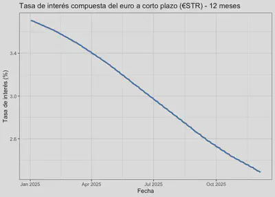
Una nueva librería: imfapi
Hace unos meses alguien de mi red en LinkedIn compartió el post de Christopher Smith donde anunciaba la creación de una nueva librería que “Proporciona funciones fáciles de usar para acceder de forma programática a datos macroeconómicos del ‘SDMX 3.0 IMF Data API’ del Fondo Monetario Internacional.”. La librería en cuestión está disponible en CRAN y funciona establemente. Además, esta librería forma parte del EconDataverse, que recomiendo explorar. A continuación voy a mostrar, de forma simplificada, como acceder a los mismos datos del WEO que vimos anteriormente.
Usando imfapi para extraer datos del WEO
En primer lugar, cargamos la librería:
library(imfapi)
Luego, extraemos los dataflows disponibles en la API del FMI:
dataflows <- imfapi::imf_get_dataflows()

dataflows |>
  dplyr::glimpse()
## Rows: 72
## Columns: 6
## $ id           <chr> "GFS_SSUC", "QGFS", "QNEA", "MFS_IR", "WHDREO", "IRFCL", …
## $ name         <chr> "GFS Statement of Sources and Uses of Cash", "Quarterly G…
## $ description  <chr> "The Government Finance Statistics (GFS) includes a cash‐…
## $ version      <chr> "10.0.0", "12.0.0", "7.0.0", "8.0.1", "5.0.0", "11.0.0", …
## $ agency       <chr> "IMF.STA", "IMF.STA", "IMF.STA", "IMF.STA", "IMF.WHD", "I…
## $ last_updated <chr> "2025-06-06T01:50:52.945047Z", "2025-09-03T16:39:57.78654…
Ahora, filtramos el dataflow WEO:
weo_flow <- dataflows |>
  dplyr::filter(id == "WEO")

weo_flow |>
  kableExtra::kable()
| id | name | description | version | agency | last_updated |
|---|---|---|---|---|---|
| WEO | World Economic Outlook (WEO) | The World Economic Outlook (WEO) database is created during the biannual WEO exercise, which begins in January and June of each year and results in the April and September/October WEO publication. Selected series from the publication are available in a database format. | 9.0.0 | IMF.RES | 2025-10-08T18:00:33.590181Z |
Y obtenemos las dimensiones del dataflow WEO:
dsd_weo <- imfapi::imf_get_datastructure(dataflow_id = "WEO")
dsd_weo |>
  kableExtra::kable()
| dimension_id | type | position |
|---|---|---|
| COUNTRY | Dimension | 0 |
| INDICATOR | Dimension | 1 |
| FREQUENCY | Dimension | 2 |
A continuación, extraemos los codelists asociados al dataflow WEO:
dim_list <- list()

for(dim_id in dsd_weo$dimension_id) {
  dim_list[[dim_id]] <- imfapi::imf_get_codelists(dimension_ids = dim_id,
                                                  dataflow_id = "WEO")
}

dim_list |>
  dplyr::bind_rows() |>
  dplyr::group_by(dimension_id) |>
  dplyr::summarise(n_codes = dplyr::n()) |>
  kableExtra::kable()
| dimension_id | n_codes |
|---|---|
| COUNTRY | 338 |
| FREQUENCY | 6 |
| INDICATOR | 145 |
En este caso tenemos 338 códigos para la dimensión COUNTRY, 6 códigos para la dimensión FREQUENCY y 145 códigos válidos para INDICATOR.
Finalmente, extraemos los datos del WEO para Bolivia y el crecimiento del PIB real:
data <- imfapi::imf_get(dataflow_id = "WEO",
                        dimensions = list(COUNTRY = "BOL",
                                          INDICATOR = "NGDP_RPCH",
                                          FREQUENCY = "A")
                        )

data |>
  kableExtra::kable()
| COUNTRY | INDICATOR | FREQUENCY | TIME_PERIOD | OBS_VALUE |
|---|---|---|---|---|
| BOL | NGDP_RPCH | A | 1980 | 0.610 |
| BOL | NGDP_RPCH | A | 1981 | 0.300 |
| BOL | NGDP_RPCH | A | 1982 | -3.939 |
| BOL | NGDP_RPCH | A | 1983 | -4.042 |
| BOL | NGDP_RPCH | A | 1984 | -0.201 |
| BOL | NGDP_RPCH | A | 1985 | -1.676 |
| BOL | NGDP_RPCH | A | 1986 | -2.574 |
| BOL | NGDP_RPCH | A | 1987 | 2.463 |
| BOL | NGDP_RPCH | A | 1988 | 2.910 |
| BOL | NGDP_RPCH | A | 1989 | 3.790 |
| BOL | NGDP_RPCH | A | 1990 | 4.636 |
| BOL | NGDP_RPCH | A | 1991 | 5.267 |
| BOL | NGDP_RPCH | A | 1992 | 1.646 |
| BOL | NGDP_RPCH | A | 1993 | 4.269 |
| BOL | NGDP_RPCH | A | 1994 | 4.667 |
| BOL | NGDP_RPCH | A | 1995 | 4.678 |
| BOL | NGDP_RPCH | A | 1996 | 4.361 |
| BOL | NGDP_RPCH | A | 1997 | 4.954 |
| BOL | NGDP_RPCH | A | 1998 | 5.029 |
| BOL | NGDP_RPCH | A | 1999 | 0.427 |
| BOL | NGDP_RPCH | A | 2000 | 2.508 |
| BOL | NGDP_RPCH | A | 2001 | 1.684 |
| BOL | NGDP_RPCH | A | 2002 | 2.486 |
| BOL | NGDP_RPCH | A | 2003 | 2.711 |
| BOL | NGDP_RPCH | A | 2004 | 4.173 |
| BOL | NGDP_RPCH | A | 2005 | 4.421 |
| BOL | NGDP_RPCH | A | 2006 | 4.797 |
| BOL | NGDP_RPCH | A | 2007 | 4.564 |
| BOL | NGDP_RPCH | A | 2008 | 6.148 |
| BOL | NGDP_RPCH | A | 2009 | 3.357 |
| BOL | NGDP_RPCH | A | 2010 | 4.127 |
| BOL | NGDP_RPCH | A | 2011 | 5.204 |
| BOL | NGDP_RPCH | A | 2012 | 5.122 |
| BOL | NGDP_RPCH | A | 2013 | 6.796 |
| BOL | NGDP_RPCH | A | 2014 | 5.461 |
| BOL | NGDP_RPCH | A | 2015 | 4.857 |
| BOL | NGDP_RPCH | A | 2016 | 4.264 |
| BOL | NGDP_RPCH | A | 2017 | 4.195 |
| BOL | NGDP_RPCH | A | 2018 | 4.224 |
| BOL | NGDP_RPCH | A | 2019 | 2.217 |
| BOL | NGDP_RPCH | A | 2020 | -8.738 |
| BOL | NGDP_RPCH | A | 2021 | 6.111 |
| BOL | NGDP_RPCH | A | 2022 | 3.606 |
| BOL | NGDP_RPCH | A | 2023 | 3.082 |
| BOL | NGDP_RPCH | A | 2024 | 0.729 |
| BOL | NGDP_RPCH | A | 2025 | 0.600 |
En la tabla anterior podemos ver los datos extraídos del WEO para Bolivia y el crecimiento del PIB real con frecuencia anual. La librería imfapi simplifica considerablemente el proceso de extracción de datos desde la API del FMI, permitiendo a los usuarios centrarse en el análisis de los datos en lugar de en los detalles técnicos de la API SDMX.
Conclusiones
El objetivo de esta entrada fue mostrar que, para el analista aplicado, trabajar con APIs SDMX no es un fin en sí mismo, sino una forma de construir flujos de trabajo más limpios, reproducibles y escalables. En lugar de depender de descargas manuales y pasos poco documentados, SDMX permite encontrar, entender y extraer datos macroeconómicos de distintos organismos bajo una lógica común.
A través del FMI y el BCE vimos que el proceso general —identificar el dataflow, revisar su estructura, consultar las codelists y finalmente extraer los datos— se repite de manera consistente, lo que facilita automatizarlo y aplicarlo a otras bases. Además, herramientas como imfapi demuestran cómo este enfoque puede simplificarse aún más, haciendo que la carga técnica sea mínima y que la mayor parte del esfuerzo se concentre en el análisis.
Estos dos modificadores le indican al servidor que queremos toda la información estructural del dataflow y todos los elementos relacionados, es decir: la DSD, los conceptos y, crucialmente, todas las codelists que dependen del dataflow. Esto nos evita tener que buscar manualmente qué codelists existen, cómo se llaman o en qué versión están. En lugar de ello, obtenemos toda la estructura completa del WEO en una sola llamada, de forma limpia y consistente. ↩︎
Por ejemplo, el dataflow
ESTque corresponde a la tasa de interés de corto plazo €STR y que se investigará más adelante se puede encontrar aquí. ↩︎