A gentle introduction to SDMX for reproducible data extraction from international organizations
This is a post I had been wanting to write for some time, and one I had promised in another similar post a few weeks ago.
When you start doing macroeconomic analysis —whether for research or for presentations— the usual workflow involves going to the data source (usually some international organization that aggregates information), downloading the dataset, and then importing it into your tool of choice to proceed with the analysis.
This workflow, however, has several drawbacks. First, it is not replicable: there are several manual steps that are not strictly documented. Moreover, it is not scalable, because if at some point a new variable becomes necessary for the analysis and was not included in the first data extraction, you need to repeat the whole process from the beginning.
Therefore, for the applied analyst, it becomes essential to automate the data extraction process, so that most of the work is focused on analysis and less on the plumbing required to gather the necessary information.
In this sense, the optimal solution is to rely on an API (application programming interface) that allows you to find, understand, and extract information quickly, so that the analysis is fully reproducible and scalable. For example, in previous posts I showed how, in a simplified way, to access the API of ECLAC and the World Economic Outlook published by the International Monetary Fund (IMF) to automate this workflow.
In this post, however, I want to broaden the data sources and present, at least conceptually, a general method that allows systematic access to data from international organizations. This is possible thanks to a standardized information model or protocol called SDMX, which allows us to access data in a more or less homogeneous way.
In what follows, I will review the SDMX model conceptually, show a relatively simplified workflow to extract information, and present some applied examples. Finally, for the IMF case, a library called imfapi has been created, which facilitates data extraction using the IMF’s SDMX API, and which I explore below.
What is SDMX?
As stated on its official website:
SDMX, which stands for Statistical Data and Metadata eXchange, is an ISO standard designed to describe statistical data and metadata, standardize their exchange, and improve their efficient distribution among statistical and similar organizations.
SDMX is sponsored by eight international organizations:
- Bank for International Settlements (BIS),
- European Central Bank (ECB),
- Statistical Office of the European Union (Eurostat),
- International Labour Organization (ILO),
- International Monetary Fund (IMF),
- Organisation for Economic Co-operation and Development (OECD),
- United Nations Statistics Division (UNSD), and
- World Bank (WB)
Each of these organizations has implemented SDMX in their statistical information systems and provides APIs following this structure. This can be seen in the table below:
| ORG | SDMX API | Documentation |
|---|---|---|
| BIS | https://stats.bis.org/api/v1 | BIS SDMX Tech Spec |
| ECB | https://data-api.ecb.europa.eu/service | ECB API Overview |
| Eurostat | https://ec.europa.eu/eurostat/api/dissemination/ | Eurostat API |
| ILO | https://sdmx.ilo.org/rest | ILOSTAT SDMX User Guide |
| IMF | https://sdmxcentral.imf.org/sdmx/v2/ | IMF Data APIs |
| OECD | https://sdmx.oecd.org/public/rest/ | OECD Data API Explainer |
| UNSD | http://data.un.org/WS/rest/ | UN SDMX / SDG API Manual |
| WB | https://api.worldbank.org/v2/sdmx/rest/ | World Bank SDMX API Queries |
Thus, analysts can access a wide range of macroeconomic and social data from different international sources using a standardized approach.
General workflow to extract SDMX data
Although each API may have its particularities and the SDMX model is quite broad, the general workflow for extracting data using SDMX APIs can be summarized in four steps. Each one corresponds to a key concept within the SDMX architecture and helps us understand how statistical agencies organize and expose their data.
Identifying the dataflow. The first step consists in identifying the dataflow. Conceptually, a dataflow is the container for a thematic dataset. It works like the “database” or the statistical domain published by an institution (for example, monetary statistics, bank balance sheets, exchange rates, or macroeconomic indicators). Identifying the appropriate dataflow involves reviewing the list of dataflows available in the API and selecting the one that contains the information relevant for the desired analysis. Without this step, it is impossible to proceed to a valid query, because every SDMX dataset starts from a specific dataflow.
Retrieving the data structure. Once the dataflow has been selected, the next step is to retrieve the associated data structure, known as the Data Structure Definition (DSD). Conceptually, the DSD is the logical schema of the dataset: it describes how observations are organized and which elements are involved in their identification. The DSD specifies the dimensions (such as country, indicator, frequency, or currency), which are key variables that classify the data and determine how they are combined to form series or observations. It also defines the main measure, which is the numerical value of the data (for example, a price index or a monetary balance), as well as additional attributes that provide contextual information (such as unit, seasonal adjustment method, or observation status). Understanding this structure is essential to know what filters can be applied and how to build the query.
Consulting the codelists. The third step consists in consulting the codelists. Each dimension defined in the DSD has an associated codelist, which is the authorized set of possible values for that dimension. Codelists act like a standard dictionary of codes that ensures interoperability between institutions and systems. For example, a codelist may contain all country codes, the types of time frequency (annual, quarterly, monthly), or the different indicators within a statistical domain. Consulting them is fundamental to know which values can be used when filtering a query and how they should be correctly encoded in the URL or request body. As we will see later, many times codelists show what is possible but not necessarily what is valid for a particular dataflow. Therefore, it is often necessary to investigate whether the DSD contains constraints on values and, if not, to resort to brute force by downloading a sample of the data and extracting unique values. In any case, the important thing is that the user becomes familiar with the data.
Extracting the data. Finally, the fourth step is to extract the data. Once we know the dataflow, its structure, and the codes allowed for each dimension, we can build a valid query to the SDMX API. This involves selecting the relevant combinations of codes (for example, country, indicator, and frequency) and applying time or detail filters as permitted by the API. The response is usually received in a standardized format, such as SDMX-JSON or SDMX-XML, which can later be processed in tools like
RorPythonfor analysis, visualization, or integration into a reproducible pipeline. This step is where all the previous work materializes, as it turns the conceptual understanding of the SDMX structure into a concrete data request.
Some examples
In this section we will work through an example using the IMF APIs and, later, the European Central Bank (ECB) APIs. Although we go step by step, the key idea is that what we are going to do is:
- Identify the available dataflows (“databases”)
- Retrieve the data structure of the dataflow of interest (“the variables”)
- Consult the codelists associated with the dimensions of interest (“the valid codes”)
- Extract the data (“the final query”)
SDMX at the IMF
The IMF provides a fairly complete collection of SDMX 3.0 APIs that give access to a wide range of macroeconomic data. These can be found, after registering, here:
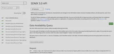
The IMF’s SDMX APIs—and in fact any SDMX 3.0 API—are designed following a hierarchical structure, where the URL acts like a path that moves from the most general to the most specific. This allows the user to progressively explore the statistical system, starting from complete catalogs and drilling down to a specific dataset or even a single time series.
The core idea is that each segment of the path adds a restriction, a filter, or a level of precision. Thus, a request can mean “show everything” or “give me exactly this data structure”, depending on how many parameters are included. Let’s go through this step by step.
Available data: the dataflow
The starting point is the base URL, which in this case is https://api.imf.org/external/sdmx/3.0. From this point we can say that the IMF API is divided into two big families: a structure family and a data family. The former allows you to explore catalogs and structures, while the latter allows you to extract specific data.
For example, if we append /structure/dataflow to the base URL, we get the complete catalog of dataflows available in the API—that is, we are asking “give me all the dataflows the IMF has”. If, on the other hand, we append /structure/datastructure, we are essentially asking “give me all the DSDs the IMF has”. This level is quite general: it does not apply any filters to the extraction, which is useful when we are not yet sure what we need.
To illustrate this, we will carry out the first step of the workflow: obtaining all the dataflows available in the IMF API and locating the dataflow corresponding to the World Economic Outlook (WEO). This can be done with the following R code:
# 1. Base URL SDMX 3.0 of the IMF
base_url <- "https://api.imf.org/external/sdmx/3.0"

# 2. Get all dataflows
flows_resp <- httr2::request(paste0(base_url, "/structure/dataflow")) |>
  httr2::req_perform()

flows_json <- flows_resp |>
  httr2::resp_body_string() |>
  jsonlite::fromJSON(flatten = TRUE)

flows <- flows_json$data$dataflows

# Dataflows table as a tibble
df_flows <- tibble::tibble(
  id      = flows$id,
  name    = flows$names.en,
  version = flows$version,
  agency  = flows$agencyID,
  dsd_urn = flows$structure
)

df_flows |>
  dplyr::select(id, name, version, agency) |>
  dplyr::arrange(id) |>
  kableExtra::kable()
| id | name | version | agency |
|---|---|---|---|
| AFRREO | Sub-Saharan Africa Regional Economic Outlook (AFRREO) | 6.0.1 | IMF.AFR |
| ANEA | National Economic Accounts (NEA), Annual Data | 6.0.1 | IMF.STA |
| APDREO | Asia and Pacific Regional Economic Outlook (APDREO) | 6.0.0 | IMF.APD |
| BOP | Balance of Payments (BOP) | 21.0.0 | IMF.STA |
| BOP_AGG | Balance of Payments and International Investment Position Statistics (BOP/IIP), World and Country Group Aggregates | 9.0.1 | IMF.STA |
| COFER | Currency Composition of Official Foreign Exchange Reserves (COFER) | 7.0.0 | IMF.STA |
| CPI | Consumer Price Index (CPI) | 5.0.0 | IMF.STA |
| CPI_WCA | Consumer Price Index (CPI), World and Country Aggregates (CPI_WCA) | 2.0.2 | IMF.STA |
| CTOT | Commodity Terms of Trade (CTOT) | 5.0.1 | IMF.RES |
| DIP | Direct Investment Positions by Counterpart Economy (formerly CDIS) | 12.0.0 | IMF.STA |
| ED | Export Diversification (ED) | 1.0.0 | IMF.RES |
| EER | Effective Exchange Rate (EER) | 6.0.0 | IMF.STA |
| EQ | Export Quality (EQ) | 2.0.0 | IMF.RES |
| ER | Exchange Rates (ER) | 4.0.1 | IMF.STA |
| FA | Fund Accounts (FA) | 8.0.0 | IMF.STA |
| FAS | Financial Access Survey (FAS) | 4.0.0 | IMF.STA |
| FD | Fiscal Decentralization (FD) | 6.0.0 | IMF.STA |
| FDI | Financial Development Index (FDI) | 1.0.0 | IMF.MCM |
| FM | Fiscal Monitor (FM) | 5.0.0 | IMF.FAD |
| FSIBSIS | Financial Soundness Indicators (FSI), Balance Sheet, Income Statement and Memorandum Series | 18.0.0 | IMF.STA |
| FSIC | Financial Soundness Indicators (FSI), Core and Additional Indicators | 13.0.1 | IMF.STA |
| FSICDM | Financial Soundness Indicators (FSI), Concentration and Distribution Measures | 7.0.0 | IMF.STA |
| GDD | Global Debt Database (GDD) | 2.0.0 | IMF.FAD |
| GFS_BS | GFS Balance Sheet | 12.0.0 | IMF.STA |
| GFS_COFOG | GFS Government Expenditures by Function | 11.0.0 | IMF.STA |
| GFS_SFCP | GFS Stocks and Flows by Counterparty | 10.0.0 | IMF.STA |
| GFS_SOEF | GFS Statement of Other Economic Flows | 11.0.0 | IMF.STA |
| GFS_SOO | GFS Statement of Operations | 12.0.0 | IMF.STA |
| GFS_SSUC | GFS Statement of Sources and Uses of Cash | 10.0.0 | IMF.STA |
| HPD | Historical Public Debt (HPD) | 1.0.0 | IMF.FAD |
| ICSD | Investment and Capital Stock Dataset (ICSD) | 1.0.0 | IMF.FAD |
| IIP | International Investment Position (IIP) | 13.0.0 | IMF.STA |
| IIPCC | Currency Composition of the International Investment Position (IIPCC) | 13.0.0 | IMF.STA |
| IL | International Liquidity (IL) | 13.0.1 | IMF.STA |
| IMTS | International Trade in Goods (by partner country) (IMTS) | 1.0.0 | IMF.STA |
| IRFCL | International Reserves and Foreign Currency Liquidity (IRFCL) | 11.0.0 | IMF.STA |
| ISORA_2016_DATA_PUB | ISORA 2016 Data | 2.0.0 | ISORA |
| ISORA_2018_DATA_PUB | ISORA 2018 Data | 2.0.0 | ISORA |
| ISORA_LATEST_DATA_PUB | ISORA Latest Data | 4.0.0 | ISORA |
| ITG | International Trade in Goods (ITG) | 4.0.0 | IMF.STA |
| ITG_WCA | International Trade in Goods, World and Country Aggregates | 2.0.4 | IMF.STA |
| ITS | International Trade in Services (ITS) | 3.0.1 | IMF.RES |
| LS | Labor Statistics (LS) | 9.0.0 | IMF.STA |
| MCDREO | Middle East and Central Asia Regional Economic Outlook (MCDREO) | 8.0.0 | IMF.MCD |
| MFS_CBS | Monetary and Financial Statistics (MFS), Central Bank Data | 24.0.0 | IMF.STA |
| MFS_DC | Monetary and Financial Statistics (MFS), Depository Corporations | 8.0.0 | IMF.STA |
| MFS_FC | Monetary and Financial Statistics (MFS), Financial Corporations | 9.0.0 | IMF.STA |
| MFS_FMP | Monetary and Financial Statistics (MFS): Financial Market Prices | 3.0.0 | IMF.STA |
| MFS_IR | Monetary and Financial Statistics (MFS), Interest Rate | 8.0.1 | IMF.STA |
| MFS_MA | Monetary and Financial Statistics (MFS), Monetary Aggregates | 10.0.1 | IMF.STA |
| MFS_NSRF | Monetary and Financial Statistics (MFS), Non-Standard Data | 1.0.3 | IMF.STA |
| MFS_ODC | Monetary and Financial Statistics (MFS), Other Depository Corporations | 10.0.0 | IMF.STA |
| MFS_OFC | Monetary and Financial Statistics (MFS), Other Financial Corporations | 7.0.0 | IMF.STA |
| MPFT | Monetary Policy Frameworks Toolkit (MPFT) | 7.0.1 | IMF.RES |
| NSDP | National Summary Data Page (NSDP) | 7.0.0 | IMF.STA |
| PCPS | Primary Commodity Price System (PCPS) | 9.0.0 | IMF.RES |
| PI | Production Indexes (PI) | 2.0.0 | IMF.STA |
| PIP | Portfolio Investment Positions by Counterpart Economy (formerly CPIS) | 4.0.0 | IMF.STA |
| PI_WCA | Production Indexes, World and Country Group Aggregates | 1.0.0 | IMF.STA |
| PPI | Producer Price Index (PPI) | 3.0.0 | IMF.STA |
| PSBS | Public Sector Balance Sheet (PSBS) | 2.0.0 | IMF.FAD |
| QGDP_WCA | Quarterly Gross Domestic Product (GDP), World and Country Aggregates | 3.0.0 | IMF.STA |
| QGFS | Quarterly Government Finance Statistics (QGFS) | 12.0.0 | IMF.STA |
| QNEA | National Economic Accounts (NEA), Quarterly Data | 7.0.0 | IMF.STA |
| SDG | IMF Reported SDG Data | 2.0.1 | IMF.STA |
| SPE | Special Purpose Entities (SPEs) | 13.0.0 | IMF.STA |
| SRD | Structural Reform Database (SRD) | 1.0.0 | IMF.RES |
| TAXFIT | Tax and Benefits Analysis Tool (TAXFIT) | 2.0.3 | IMF.RES |
| TEG | Trade in Low Carbon Technology Goods (TEG) | 3.0.2 | IMF.STA |
| WEO | World Economic Outlook (WEO) | 9.0.0 | IMF.RES |
| WHDREO | Western Hemisphere Regional Economic Outlook (WHDREO) | 5.0.0 | IMF.WHD |
| WPCPER | Crypto-based Parallel Exchange Rates (Working Paper dataset WP-CPER) | 6.0.0 | IMF.STA |
In the table above we can see all the dataflows available in the IMF API. Each dataflow has a unique identifier (id), a descriptive name (name), a version (version), a responsible agency (agency), and a URN (Uniform Resource Name) not shown in the previous table but pointing to its associated data structure (dsd_urn).
In our case we are interested in the WEO dataflow. We can filter the dataflow of interest as follows:
# Keep only the WEO dataflow
weo <- df_flows |>
  dplyr::filter(id == "WEO")

weo |>
  kableExtra::kable()
| id | name | version | agency | dsd_urn |
|---|---|---|---|---|
| WEO | World Economic Outlook (WEO) | 9.0.0 | IMF.RES | urn:sdmx:org.sdmx.infomodel.datastructure.DataStructure=IMF.RES:DSD_WEO(9.0+.0) |
Data structure: the dimensions
Now that we have the dataflow of interest, the next step is to understand which variables (dimensions) are available in its data structure. To do this, the API we need to query has the following form: /structure/datastructure/{agency}/{dsd_id}/{version}, where {agency}, {dsd_id}, and {version} are the components we must extract from the WEO dataflow URN. Note that if we do not specify these three fields, we run the risk of getting outdated information.
How do we obtain this information? The good thing is that, when we query the dataflow, this information is contained in the associated URN:
# Parse the URN of WEO's datastructure
urn <- weo$dsd_urn
urn
## [1] "urn:sdmx:org.sdmx.infomodel.datastructure.DataStructure=IMF.RES:DSD_WEO(9.0+.0)"
Note that here we have the three essential pieces:
- The agency responsible for the DSD:
IMF.RES - The DSD identifier:
DSD_WEO - The DSD version:
9.0+.0
To systematically extract these pieces we can use regular expressions in R as follows:
m     <- base::regexec("DataStructure=([^:]+):([^()]+)\\(([^)]+)\\)", urn)
parts <- base::regmatches(urn, m)[[1]]

agency_dsd  <- parts[2]   # e.g. "IMF.RES"
dsd_id      <- parts[3]   # e.g. "DSD_WEO"
version_dsd <- parts[4]   # e.g. "9.0+.0"

# Download WEO's datastructure and inspect dimensions
dsd_url <- paste0(
  base_url,
  "/structure/datastructure/",
  agency_dsd, "/", dsd_id, "/", version_dsd
)
dsd_url
## [1] "https://api.imf.org/external/sdmx/3.0/structure/datastructure/IMF.RES/DSD_WEO/9.0+.0"
Now that we have the URL for WEO’s datastructure, we can download it and inspect the available dimensions:
dsd_resp <- httr2::request(dsd_url) |>
  httr2::req_perform()

dsd_json <- dsd_resp |>
  httr2::resp_body_string() |>
  jsonlite::fromJSON(flatten = TRUE)

# "Regular" dimensions: COUNTRY, INDICATOR, FREQUENCY
dims_main <- dsd_json$data$dataStructures$dataStructureComponents.dimensionList.dimensions[[1]] |>
  tibble::as_tibble() |>
  dplyr::select(position, id, type)

# Time dimension: TIME_PERIOD
time_dim <- dsd_json$data$dataStructures$dataStructureComponents.dimensionList.timeDimensions[[1]] |>
  tibble::as_tibble() |>
  dplyr::select(position, id, type)

# Full dimension order
dims_clean <- dplyr::bind_rows(dims_main, time_dim) |>
  dplyr::arrange(position)

dims_clean |>
  kableExtra::kable()
| position | id | type |
|---|---|---|
| 0 | COUNTRY | Dimension |
| 1 | INDICATOR | Dimension |
| 2 | FREQUENCY | Dimension |
| 3 | TIME_PERIOD | TimeDimension |
In the table above we can see the available dimensions in the WEO dataflow (COUNTRY, INDICATOR, FREQUENCY, and TIME_PERIOD). These dimensions are key for understanding how the data are organized and what filters we can apply when extracting specific information.
Note also that, although the query ran without errors, we first explored dsd_json to understand where and how the information was stored.
Codelists: the valid codes
As a third step, and before extracting data, it is important to know the valid codes for each dimension of the dataset. This is essential because, when building the final query, we must make sure to use the exact values that the API recognizes. Otherwise, it will return an error. For example, if we want to obtain real GDP growth for a specific country, we need to know how the IMF codes the country, the indicator, and the frequency. It is not enough to write “Bolivia” or “Real GDP growth”: we must use the official codes defined by the dataset’s structure.
Each of the WEO dimensions—COUNTRY, INDICATOR, FREQUENCY, and TIME_PERIOD—has an authorized set of possible values: the codelist. For example, country codes might be BOL, ARG, or USA; indicators could be NGDP_RPCH, LUR, and so on; and valid frequencies are typically A (annual), Q (quarterly), etc. An important detail is that each dataset can have different codelists, even for conceptually similar items. The IMF might use one list of countries for WEO, another for BOP (Balance of Payments), and another for monetary statistics. This means that codes that work for one dataflow will not necessarily work for another.
Therefore, if we want to query WEO data, we cannot make up codes or rely on old lists: we need to query the official codelists from the IMF. The only safe way to do this is to start from the dataflow, retrieve its structure (the DSD), and from there obtain the correct lists of codes for each dimension. This procedure ensures that the query is reproducible, accurate, and fully compatible with the IMF’s internal definitions.
To obtain the codelists associated with the WEO dataflow, we use a specific URL from the IMF’s SDMX API. The general pattern is: /structure/dataflow/{agency}/{dataflow_id}/+, where {agency} and {dataflow_id} come from the dataflow itself (IMF.RES and WEO, respectively, in our case). The + symbol indicates that we want the latest available version. But the most important part is the parameters we add at the end: ?detail=full&references=descendants1.
For our case, the full URL to obtain WEO’s codelists is:
weo_struct_url <- paste0(
  base_url,
  "/structure/dataflow/",
  weo$agency, "/", weo$id, "/+",
  "?detail=full&references=descendants"
)
weo_struct_url
## [1] "https://api.imf.org/external/sdmx/3.0/structure/dataflow/IMF.RES/WEO/+?detail=full&references=descendants"
When we send a request to this URL, we get a response that includes all the codelists associated with the WEO dataflow. We can process this response to extract the specific codelists we need for each dimension:
weo_struct_resp <- httr2::request(weo_struct_url) |>
  httr2::req_perform()

weo_struct_json <- weo_struct_resp |>
  httr2::resp_body_string() |>
  jsonlite::fromJSON(flatten = TRUE)

# Codelists table
codelists_tbl <- weo_struct_json$data$codelists

codelists_tbl |>
  dplyr::select(id, name, version, agencyID) |>
  head() |>
  kableExtra::kable()
| id | name | version | agencyID |
|---|---|---|---|
| CL_SEC_CLASSIFICATION | Security Classification | 1.0.1 | IMF |
| CL_METHODOLOGY | Methodology | 2.6.0 | IMF |
| CL_DEPARTMENT | Department | 1.0.2 | IMF |
| CL_COUNTRY | Country | 1.5.1 | IMF |
| CL_TOPIC | Topic | 2.2.0 | IMF |
| CL_UNIT_MULT | Unit Multiplier | 1.0.2 | IMF |
Note that in the table above we have extracted quite a bit of information about the codelists available for the WEO dataflow. In the following code, we summarize what we obtained:
# Summary view of the codelists
weo_codelists_overview <- tibble::tibble(
  cl_id   = codelists_tbl$id,
  cl_name = ifelse(is.na(codelists_tbl$names.en),
                   yes = codelists_tbl$name,
                   no = codelists_tbl$names.en
                   ),
  n_codes = sapply(codelists_tbl$codes, nrow)
)

weo_codelists_overview |>
  dplyr::arrange(desc(cl_id)) |>
  kableExtra::kable()
| cl_id | cl_name | n_codes |
|---|---|---|
| CL_WEO_INDICATOR | World Economic Outlook (WEO) Indicator | 145 |
| CL_WEO_COUNTRY | World Economic Outlook (WEO) Country | 338 |
| CL_VALUATION | Valuation | 26 |
| CL_UNIT_MULT | Unit Multiplier | 31 |
| CL_UNIT | Unit of Measure | 270 |
| CL_TRANSFORMATION | Transformation | 487 |
| CL_TRADE_FLOW | Trade flow | 50 |
| CL_TOPIC | Topic | 118 |
| CL_S_ADJUSTMENT | Seasonal Adjustment | 17 |
| CL_STATISTICAL_MEASURES | Statistical Measures | 23 |
| CL_SOC_CONCEPTS | Social Concepts | 31 |
| CL_SEX | Sex | 9 |
| CL_SEC_CLASSIFICATION | Security Classification | 6 |
| CL_SECTOR | Institutional Sector | 288 |
| CL_REPORTING_PERIOD_TYPE | REPORTING_PERIOD_TYPE | 6 |
| CL_PRICES | Prices | 15 |
| CL_OVERLAP | IMF Data Overlap | 1 |
| CL_ORGANIZATION | Organization | 1588 |
| CL_OBS_STATUS | Observation Status | 22 |
| CL_NA_STO | NA Stocks, Transactions, Other Flows | 636 |
| CL_MFS_INSTR | Monetary and Financial Instruments | 18 |
| CL_METHODOLOGY | Methodology | 69 |
| CL_LANGUAGE | Language | 93 |
| CL_INT_TTC | Interest Rate types, terms and conditions | 101 |
| CL_INT_ACC_ITEM | International accounts item | 507 |
| CL_INSTR_ASSET | Instrument and assets classification | 342 |
| CL_INDEX_TYPE | Index type | 49 |
| CL_GFS_STO | GFS Stocks, Transactions, Other Flows | 389 |
| CL_GENDER | Gender | 15 |
| CL_FUNCTIONAL_CAT | Functional category | 72 |
| CL_FSENTRY | Flow or stock entry | 43 |
| CL_FREQ | Frequency | 6 |
| CL_FI_MATURITY | Maturity of Financial Instrument | 32 |
| CL_EXRATE | Exchange Rate | 37 |
| CL_DERIVATION_TYPE | Derivation Type | 12 |
| CL_DEPARTMENT | Department | 34 |
| CL_DECIMALS | Decimals | 16 |
| CL_CURRENCY | Currency | 177 |
| CL_COUNTRY | Country | 337 |
| CL_CONF_STATUS | Confidentiality Status | 12 |
| CL_COMMODITY | Commodity | 135 |
| CL_COICOP_2018 | COICOP 2018 | 16 |
| CL_COICOP_1999 | COICOP 1999 | 15 |
| CL_COFOG | COFOG | 190 |
| CL_CIVIL_STATUS | Civil (or Marital) Status | 8 |
| CL_ACCOUNTS | Macroeconomic and financial accounts | 40 |
| CL_ACCOUNTING_ENTRY | Accounting Entry | 82 |
| CL_ACCESS_SHARING_LEVEL | Access and Sharing Level | 8 |
In the table above we can see a summary of the codelists available for the WEO dataflow. Each codelist has an identifier (cl_id), a descriptive name (cl_name), and the number of codes it contains (n_codes). In our case, we are particularly interested in the codelists associated with the COUNTRY, INDICATOR, and FREQUENCY dimensions: CL_WEO_COUNTRY, CL_WEO_INDICATOR, and CL_FREQUENCY.
For example, for CL_WEO_COUNTRY:
weo_country_codes <- codelists_tbl$codes[[which(codelists_tbl$id == "CL_WEO_COUNTRY")]] |>
  tibble::as_tibble() |>
  dplyr::transmute(
    code    = id,
    name_en = names.en  # in CL_WEO_COUNTRY it appears as names.en1
  )
weo_country_codes |>
  head(20) |>
  kableExtra::kable()
| code | name_en |
|---|---|
| GX123 | Other Advanced Economies (Advanced Economies excluding G7 and Euro Area countries) |
| AFG | Afghanistan, Islamic Republic of |
| ALB | Albania |
| DZA | Algeria |
| ASM | American Samoa |
| AND | Andorra, Principality of |
| AGO | Angola |
| AIA | Anguilla, United Kingdom-British Overseas Territory |
| ATG | Antigua and Barbuda |
| ARG | Argentina |
| ARM | Armenia, Republic of |
| ABW | Aruba, Kingdom of the Netherlands |
| AUS | Australia |
| AUT | Austria |
| AZE | Azerbaijan, Republic of |
| BHS | Bahamas, The |
| BHR | Bahrain, Kingdom of |
| BGD | Bangladesh |
| BRB | Barbados |
| BLR | Belarus, Republic of |
In the table above we can see the valid country codes for the WEO dataflow. Each country has a code (code) and an English name (name_en). These codes are essential for building precise queries to the IMF API.
Next, we look for the available INDICATOR codes in WEO:
weo_indicator_codes <- codelists_tbl$codes[[which(codelists_tbl$id == "CL_WEO_INDICATOR")]] |>
  tibble::as_tibble() |>
  dplyr::transmute(
    code    = id,
    name_en = names.en
  )

weo_indicator_codes |>
  kableExtra::kable()
| code | name_en |
|---|---|
| LUR | Unemployment rate |
| PCOALSA | Coal, South Africa, Export price, US dollars per metric tonne |
| DSP | External debt: total debt service, amortization, US dollar |
| DSI | External debt: total debt service, interest, US dollar |
| DSP_NGDPD | External debt: total debt service, amortization, Percent of GDP |
| BX | Exports of goods and services, US dollar |
| BM | Imports of goods and services, US dollar |
| DS | External debt: total debt service, US dollar |
| TTPCH | Terms of trade of goods and services, percent change |
| DSI_NGDPD | External debt: total debt service, interest, Percent of GDP |
| NGDP_RPCHMK | Gross domestic product (GDP), Constant prices, Percent |
| NGDPD | Gross domestic product (GDP), Current prices, US dollar |
| PTEA | Tea, Kenyan, Unit prices, US cents per kilogram |
| DS_NGDPD | External debt: total debt service, Percent of GDP |
| D | External debt, US dollar |
| NGDP_D | Gross domestic product (GDP), Price deflator, Index |
| NGDP_RPCH | Gross domestic product (GDP), Constant prices, Percent change |
| TTTPCH | Terms of trade of goods, percent change |
| NGDP_R | Gross domestic product (GDP), Constant prices, Domestic currency |
| NGDP | Gross domestic product (GDP), Current prices, Domestic currency |
| NGSD_NGDP | Gross national savings, Percent of GDP |
| PSUNO | Sunflower oil, Export price, US dollars per metric tonne |
| PNGASEU | Natural gas, EU, Unit prices, US dollars per million metric British thermal units of gas |
| PZINC | Zinc, Unit prices, US dollars per metric tonne |
| PPPSH | Gross domestic product (GDP), Purchasing power parity (PPP) international dollar, percent of world GDP, Percent, ICP benchmarks 2017-2021 |
| D_NGDPD | External debt, Percent of GDP |
| PPPPC | Gross domestic product (GDP), Per capita, purchasing power parity (PPP) international dollar, ICP benchmarks 2017-2021 |
| PPPGDP | Gross domestic product (GDP), Current prices, Purchasing power parity (PPP) international dollar, ICP benchmarks 2017-2021 |
| DSP_BX | External debt: total debt service, amortization, Percent of exports of goods and services |
| PPORK | Swine, Unit prices, US cents per pound |
| PSAWMAL | Hard sawnwood, Dark Red Meranti, Unit prices, US dollars per cubic meter |
| PORANG | Orange, Import price, US dollars per metric tonne |
| PTIN | Tin, Unit prices, US dollars per metric tonne |
| PPOULT | Poultry, Unit prices, US cents per pound |
| DSI_BX | External debt: total debt service, interest, Percent of exports of goods and services |
| NGDPDPC | Gross domestic product (GDP), Current prices, Per capita, US dollar |
| PSAWORE | Soft sawnwood, Export price, US dollars per cubic meter |
| PROIL | Rapeseed oil, Unit prices, US dollars per metric tonne |
| PLAMB | Lamb, Unit prices, US cents per pound |
| PBARL | Barley, Unit prices, US dollars per metric tonne |
| PLOGORE | Soft logs, Export price, US dollars per cubic meter |
| GGR_NGDP | Revenue, General government, Percent of GDP |
| TRADEPCH | Trade of goods and services, Volume, Percent change |
| PALUM | Aluminum, Unit prices, US dollars per metric tonne |
| PLOGSK | Hard logs, import price Japan, Import price, US dollars per cubic meter |
| PWOOLC | Wool, coarse, Unit prices, US cents per kilogram |
| GGXWDN_NGDP | Net debt, General government, Percent of GDP |
| PFISH | Fishmeal, Unit prices, US dollars per metric tonne |
| NGDPRPC | Gross domestic product (GDP), Constant prices, Per capita, Domestic currency |
| PNGASJP | LNG, Asia, Unit prices, US dollars per million metric British thermal units of gas |
| LE | Employed persons, Persons for countries / Index for country groups |
| NGDPPC | Gross domestic product (GDP), Current prices, Per capita, Domestic currency |
| GGR | Revenue, General government, Domestic currency |
| PWOOLF | Wool, fine, Unit prices, US cents per kilogram |
| PCOFFOTM | Coffee, other mild Arabica, Unit prices, US cents per pound |
| PNICK | Nickel, Unit prices, US dollars per metric tonne |
| BCA | Current account balance (credit less debit), US dollar |
| PBANSOP | Bananas, Unit prices, US dollars per metric tonne |
| PRICENPQ | Rice, Thailand, Unit prices, US dollars per metric tonne |
| DS_BX | External debt: total debt service, Percent of exports of goods and services |
| PCOFFROB | Coffee, Robustas, Unit prices, US cents per pound |
| PSALM | Fish, Export price, US dollars per kilogram |
| PSUGAUSA | Sugar, No. 16, US, Import price, US cents per pound |
| GGXWDG_NGDP | Gross debt, General government, Percent of GDP |
| PCOPP | Copper, Unit prices, US dollars per metric tonne |
| PLEAD | Lead, Unit prices, US dollars per metric tonne |
| PBEEF | Beef, Import price, US cents per pound |
| BF | Financial account balance (assets less liabilities), US dollar |
| PURAN | Uranium, Unit prices, US dollars per pound |
| BCA_NGDPD | Current account balance (credit less debit), Percent of GDP |
| PHIDE | Hides, Unit prices, US cents per pound |
| PGNUTS | Groundnuts, Unit prices, US dollars per metric tonne |
| GGSB | Structural balance, General government, Domestic currency |
| BFP | Portfolio investment, Net (assets minus liabilities), US dollar |
| GGX_NGDP | Expenditure, General government, Percent of GDP |
| GGXWDG | Gross debt, General government, Domestic currency |
| GGXWDN | Net debt, General government, Domestic currency |
| NGDP_FY | Gross domestic product (GDP), Current prices, Fiscal year, Domestic currency |
| GGX | Expenditure, General government, Domestic currency |
| PRUBB | Rubber, Unit prices, US cents per pound |
| PWHEAMT | Wheat, Unit prices, US dollars per metric tonne |
| PMAIZMT | Corn, Unit prices, US dollars per metric tonne |
| GGSB_NPGDP | Structural balance, General government, Percent |
| POLVOIL | Olive oil, Unit prices, US dollars per metric tonne |
| PIORECR | Iron ore, Unit prices, US dollars per metric tonne |
| D_BX | External debt, Percent of exports of goods and services |
| BFD | Direct investment, Net (assets minus liabilities), US dollar |
| TX_RPCH | Exports of goods and services, Volume, Free on board (FOB), Percent change |
| PCOCO | Cocoa, Unit prices, US dollars per metric tonne |
| BFO | Other investment, Net (assets minus liabilities), US dollar |
| PPOIL | Palm oil, Unit prices, US dollars per metric tonne |
| NGDPRPPPPC | Gross domestic product (GDP), Constant prices, Per capita, purchasing power parity (PPP) international dollar, ICP benchmark 2021 |
| PRAWMW | Agricultural raw materials, Commodity price index |
| PSMEA | Soybean meal, Unit prices, US dollars per metric tonne |
| PCOTTIND | Cotton, Unit prices, US cents per pound |
| PCOALAU | Coal, Australia, Unit prices, US dollars per metric tonne |
| PNGASUS | Natural Gas, US Henry Hub Gas, Unit prices, US dollars per metric tonne |
| TXGM_D | Exports of manufactures, Price deflator, Free on board (FOB), Index |
| TM_RPCH | Imports of goods and services, Volume, Cost insurance freight (CIF), Percent change |
| PSOIL | Soybeans oil, Unit prices, US dollars per metric tonne |
| PSUGAISA | Sugar, No. 11, World, Unit prices, US cents per pound |
| BFF | Financial derivatives and employee stock options, Net (assets minus liabilities), US dollar |
| NGAP_NPGDP | Output gap, Percent of potential GDP |
| PSOYB | Soybeans, Unit prices, US dollars per metric tonne |
| PINDUW | Industrial materials, Commodity price index |
| GGXCNL | Net lending (+) / net borrowing (-), General government, Domestic currency |
| BFRA | Change in reserve assets, Net (assets minus liabilities), US dollar |
| TXGM_DPCH | Exports of manufactures, Price deflator, Free on board (FOB), Percent change |
| POILBRE | Brent crude, Unit prices, US dollars per barrel |
| PSHRI | Shrimp, Unit prices, US dollars per kilogram |
| GGXCNL_NGDP | Net lending (+) / net borrowing (-), General government, Percent of GDP |
| PCOALW | Coal, Commodity price index |
| PBEVEW | Beverages, Commodity price index |
| PWOOLW | Wool, Commodity price index |
| POILDUB | Dubai crude, Unit prices, US dollars per barrel |
| POILWTI | WTI crude, Unit prices, US dollars per barrel |
| PCOFFW | Coffee, Commodity price index |
| PCPI | All Items, Consumer price index (CPI), Period average |
| PSEAFW | Seafood, Commodity price index |
| PTIMBW | Timber, Commodity price index |
| GGXONLB_NGDP | Primary net lending (+) / net borrowing (-), General government, Percent of GDP |
| PSUGAW | Sugar, Commodity price index |
| POILAPSP | APSP crude oil, Unit prices, US dollars per barrel |
| PCEREW | Cereal, Commodity price index |
| PALLFNFW | All commodities, Commodity price index |
| PCPIE | All Items, Consumer price index (CPI), End-of-period (EoP) |
| GGXONLB | Primary net lending (+) / net borrowing (-), General government, Domestic currency |
| TXG_RPCH | Exports of goods, Volume, Free on board (FOB), Percent change |
| TMG_RPCH | Imports of goods, Volume, Cost insurance freight (CIF), Percent change |
| PSOFTW | Softwood, Commodity price index |
| PHARDW | Hardwood, Commodity price index |
| PCPIPCH | All Items, Consumer price index (CPI), Period average, percent change |
| PMEATW | Meat, Commodity price index |
| PFANDBW | Food and beverage, Commodity price index |
| PCPIEPCH | All Items, Consumer price index (CPI), End-of-period (EoP), percent change |
| PNFUELW | Non-fuel, Commodity price index |
| PNRGW | Energy, Commodity price index |
| LP | Population, Persons for countries / Index for country groups |
| PNGASW | Natural gas, Commodity price index |
| PPPEX | Rate, Domestic currency per international dollar in PPP terms, ICP benchmarks 2017-2021 |
| PFOODW | Food, Commodity price index |
| PMETAW | Metal, Commodity price index |
| POILAPSPW | APSP crude oil, Commodity price index |
| NID_NGDP | Gross capital formation, Percent of GDP |
| PVOILW | Vegetable oil, Commodity price index |
Finally, for the frequency:
weo_frequency_codes <- codelists_tbl$codes[[which(codelists_tbl$id =="CL_FREQ")]] |>
  tibble::as_tibble() |>
  dplyr::transmute(
    code    = id,
    name_en = names.en
  )
weo_frequency_codes |>
  kableExtra::kable()
| code | name_en |
|---|---|
| A | Annual |
| D | Daily |
| M | Monthly |
| Q | Quarterly |
| S | Half-yearly, semester |
| W | Weekly |
Once we have the valid codes for the dimensions of interest, we are ready to proceed to the extraction of specific data from the WEO dataflow. This is the final step of the SDMX workflow and will allow us to obtain the time series needed for our macroeconomic analysis.
Extracting data: the final query
With valid codes in hand for the COUNTRY, INDICATOR, and FREQUENCY dimensions, we are now in a position to build the final query to extract specific data from the WEO dataflow. From the IMF API’s perspective, the general data endpoint has the form:
/data/{context}/{agencyID}/{resourceID}/{version}/{key}[?c]
In our case, {context} will be dataflow, {agencyID} will be IMF.RES, {resourceID} will be WEO, and {version} will be the latest stable version (+). That is, everything before {key} is already known from the previous steps. What we still need to define is the key and, optionally, the filter parameter c.
The key parameter is the central piece of the query: it represents the combination of dimension values that identifies a series or a subset of the “cube” of data. The API defines it as “the combination of dimension values identifying series or slices of the cube”. In practice, this translates into a string where dimension values are concatenated following the order defined in the DSD.
In the case of WEO, we saw that the order is COUNTRY.INDICATOR.FREQUENCY, so a key like BOL.NGDP_RPCH.A means: country Bolivia (BOL), indicator “Real GDP, percent change” (NGDP_RPCH), and annual frequency (A). The API also allows the use of wildcards (*), for example BOL.*.A (all annual series for Bolivia) or *.NGDP_RPCH.A (annual real GDP growth for all countries). This makes the key a very compact way of specifying which dimension combinations we want.
The c parameter, in turn, allows additional filtering using a syntax like c[DIM]=value. The documentation describes it as “Filter data by component value (e.g. c[FREQ]=A)”, and it also allows logical operators. In our simple example, we do not use c because we already restrict country, indicator, and frequency directly in the key, and we let the API return the full history of the series. However, c is very useful when you want to apply additional filters (for example, narrowing the time range, selecting only certain currencies, methods, or observation statuses) without complicating the key, or when you are working with richer dimensional structures.
Suppose we want to obtain real GDP growth (percent change) for Bolivia at annual frequency.
# Code for Bolivia (according to the WEO codelist)
bol_code <- "BOL"

# Code for the "Real GDP, percent change" indicator
rgdp_code <- "NGDP_RPCH"

# Annual frequency (A) according to the FREQUENCY dimension
freq_code <- "A"

# SDMX key for WEO: COUNTRY.INDICATOR.FREQUENCY
weo_key <- paste(bol_code, rgdp_code, freq_code, sep = ".")
weo_key
## [1] "BOL.NGDP_RPCH.A"
Now that we have the key, we proceed to make the query:
# SDMX 3.0 data extraction URL (correct data query)
weo_data_url <- paste0(
  base_url,
  "/data/dataflow/",
  weo$agency, "/", weo$id, "/+/",
  weo_key
)

weo_data_resp <- httr2::request(weo_data_url) |>
  httr2::req_url_query(
    dimensionAtObservation = "TIME_PERIOD",
    attributes             = "dsd",
    measures               = "all",
    includeHistory         = "false"
  ) |>
  httr2::req_perform()

weo_data_json <- weo_data_resp |>
  httr2::resp_body_string() |>
  jsonlite::fromJSON(flatten = FALSE)
In weo_data_json we have the full API response containing the requested data. The structure of this object is quite complex, as it is a list of lists with several different levels of depth.
str(weo_data_json, max.level = 4)
## List of 2
##  $ meta: Named list()
##  $ data:List of 2
##   ..$ dataSets  :'data.frame':	1 obs. of  4 variables:
##   .. ..$ structure               : int 0
##   .. ..$ action                  : chr "Replace"
##   .. ..$ series                  :'data.frame':	1 obs. of  1 variable:
##   .. .. ..$ 0:0:0:'data.frame':	1 obs. of  2 variables:
##   .. ..$ dimensionGroupAttributes:'data.frame':	1 obs. of  1 variable:
##   .. .. ..$ :0:::List of 1
##   ..$ structures:'data.frame':	1 obs. of  6 variables:
##   .. ..$ dataSets   :List of 1
##   .. .. ..$ : int 0
##   .. ..$ links      :List of 1
##   .. .. ..$ :'data.frame':	2 obs. of  2 variables:
##   .. ..$ dimensions :'data.frame':	1 obs. of  2 variables:
##   .. .. ..$ series     :List of 1
##   .. .. ..$ observation:List of 1
##   .. ..$ measures   :'data.frame':	1 obs. of  1 variable:
##   .. .. ..$ observation:List of 1
##   .. ..$ attributes :'data.frame':	1 obs. of  3 variables:
##   .. .. ..$ dimensionGroup:List of 1
##   .. .. ..$ series        :List of 1
##   .. .. ..$ observation   :List of 1
##   .. ..$ annotations:List of 1
##   .. .. ..$ : list()
The next step, therefore, is to transform this response into a more manageable format, such as a tibble in R that contains time observations and their corresponding values. First, we extract the dataSets object from the previous list and everything it contains:
# Series 0:0:0 (the only one we requested in WEO)
obs_df <- weo_data_json$data$dataSets$series$`0:0:0`$observations

obs_values <- obs_df[1, ] |>
  unlist(use.names = FALSE) |>
  as.numeric()

# TIME_PERIOD from the structure
time_dim    <- weo_data_json$data$structures$dimensions$observation[[1]]$values |>
  unlist(use.names = FALSE)

# Final tibble (year, value)
weo_bol_rgdp <- tibble::tibble(
  time  = as.integer(time_dim),
  value = obs_values
) |>
  dplyr::arrange(time)

weo_bol_rgdp |>
  kableExtra::kable()
| time | value |
|---|---|
| 1980 | 0.610 |
| 1981 | 0.300 |
| 1982 | -3.939 |
| 1983 | -4.042 |
| 1984 | -0.201 |
| 1985 | -1.676 |
| 1986 | -2.574 |
| 1987 | 2.463 |
| 1988 | 2.910 |
| 1989 | 3.790 |
| 1990 | 4.636 |
| 1991 | 5.267 |
| 1992 | 1.646 |
| 1993 | 4.269 |
| 1994 | 4.667 |
| 1995 | 4.678 |
| 1996 | 4.361 |
| 1997 | 4.954 |
| 1998 | 5.029 |
| 1999 | 0.427 |
| 2000 | 2.508 |
| 2001 | 1.684 |
| 2002 | 2.486 |
| 2003 | 2.711 |
| 2004 | 4.173 |
| 2005 | 4.421 |
| 2006 | 4.797 |
| 2007 | 4.564 |
| 2008 | 6.148 |
| 2009 | 3.357 |
| 2010 | 4.127 |
| 2011 | 5.204 |
| 2012 | 5.122 |
| 2013 | 6.796 |
| 2014 | 5.461 |
| 2015 | 4.857 |
| 2016 | 4.264 |
| 2017 | 4.195 |
| 2018 | 4.224 |
| 2019 | 2.217 |
| 2020 | -8.738 |
| 2021 | 6.111 |
| 2022 | 3.606 |
| 2023 | 3.082 |
| 2024 | 0.729 |
| 2025 | 0.600 |
Finally, we can also make a richer query. For example, we can extract both real GDP growth and the primary deficit as a percentage of GDP for Bolivia, Spain, and the United States between 2015 and 2025:
# 1. Query parameters

countries  <- c("BOL", "ESP", "USA")
indicators <- c("NGDP_RPCH", "GGXONLB_NGDP")  # Real GDP % and deficit % of GDP
freq_code  <- "A"                             # Annual frequency

country_key   <- paste(countries,  collapse = "+")
indicator_key <- paste(indicators, collapse = "+")
weo_key_multi <- paste(country_key, indicator_key, freq_code, sep = ".")

# SDMX 3.0 data URL (IMF WEO)
weo_data_url_multi <- paste0(
  base_url,
  "/data/dataflow/",
  weo$agency, "/", weo$id, "/+/",
  weo_key_multi
)


# 2. API call (1980–2030)

weo_data_resp_multi <- httr2::request(weo_data_url_multi) |>
  httr2::req_url_query(
    dimensionAtObservation = "TIME_PERIOD",
    attributes             = "dsd",
    measures               = "all",
    includeHistory         = "false",
    startPeriod            = "1980",
    endPeriod              = "2030"
  ) |>
  httr2::req_perform()

weo_data_json_multi <- weo_data_resp_multi |>
  httr2::resp_body_string() |>
  jsonlite::fromJSON(flatten = FALSE)


# 3. Dimension structures

series_dims_resp <- weo_data_json_multi$data$structures$dimensions$series[[1]]
obs_dim_resp     <- weo_data_json_multi$data$structures$dimensions$observation[[1]]

time_values <- obs_dim_resp$values |>
  unlist(use.names = FALSE)


# 4. Extract the series

series_df <- weo_data_json_multi$data$dataSets$series

# Each element is a data.frame with $attributes and $observations
series_list <- lapply(series_df, function(col) col$observations)
names(series_list) <- names(series_df)

# Function to unnest a series
extract_series_tbl <- function(obs_df, series_name) {
  # Dimension indices from "0:0:0"
  idx <- as.integer(strsplit(series_name, ":", fixed = TRUE)[[1]]) + 1L

  # Map indices to COUNTRY / INDICATOR / FREQUENCY codes
  dim_values <- purrr::map2_chr(
    seq_along(series_dims_resp$id),
    idx,
    ~ series_dims_resp$values[[.x]]$id[.y]
  )
  names(dim_values) <- series_dims_resp$id

  # Number of observations
  n_obs <- ncol(obs_df)
  if (is.null(n_obs) || n_obs == 0) {
    return(tibble::tibble(
      COUNTRY     = character(0),
      INDICATOR   = character(0),
      FREQ        = character(0),
      TIME_PERIOD = integer(0),
      value       = numeric(0)
    ))
  }

  # Map column names "0,1,2,...,41,..." to time_values indices
  pos_idx     <- as.integer(colnames(obs_df)) + 1L
  these_times <- as.integer(time_values[pos_idx])

  values_num <- obs_df[1, ] |>
    unlist(use.names = FALSE) |>
    as.numeric()

  tibble::tibble(
    COUNTRY     = dim_values[["COUNTRY"]],
    INDICATOR   = dim_values[["INDICATOR"]],
    FREQ        = dim_values[["FREQUENCY"]],
    TIME_PERIOD = these_times,
    value       = values_num
  )
}

# Apply to all series
weo_multi_tidy_raw <- purrr::imap_dfr(
  series_list,
  extract_series_tbl
)


# 5. Filter 2015–2025

weo_multi_tidy <- weo_multi_tidy_raw |>
  dplyr::filter(TIME_PERIOD >= 2015, TIME_PERIOD <= 2025) |>
  dplyr::arrange(COUNTRY, INDICATOR, TIME_PERIOD)

# Wide version (one column per indicator)
weo_multi_wide <- weo_multi_tidy |>
  tidyr::pivot_wider(
    id_cols    = c(COUNTRY, TIME_PERIOD),
    names_from  = INDICATOR,
    values_from = value
  )

weo_multi_wide |>
  kableExtra::kable()
| COUNTRY | TIME_PERIOD | GGXONLB_NGDP | NGDP_RPCH |
|---|---|---|---|
| BOL | 2015 | -5.934 | 4.857 |
| BOL | 2016 | -6.253 | 4.264 |
| BOL | 2017 | -6.743 | 4.195 |
| BOL | 2018 | -6.979 | 4.224 |
| BOL | 2019 | -5.875 | 2.217 |
| BOL | 2020 | -11.228 | -8.738 |
| BOL | 2021 | -7.979 | 6.111 |
| BOL | 2022 | -5.499 | 3.606 |
| BOL | 2023 | -8.671 | 3.082 |
| BOL | 2024 | -7.506 | 0.729 |
| BOL | 2025 | -9.934 | 0.600 |
| ESP | 2015 | -2.675 | 4.061 |
| ESP | 2016 | -1.885 | 2.915 |
| ESP | 2017 | -0.866 | 2.896 |
| ESP | 2018 | -0.399 | 2.395 |
| ESP | 2019 | -1.001 | 1.961 |
| ESP | 2020 | -7.999 | -10.940 |
| ESP | 2021 | -4.723 | 6.683 |
| ESP | 2022 | -2.536 | 6.370 |
| ESP | 2023 | -1.731 | 2.461 |
| ESP | 2024 | -1.335 | 3.455 |
| ESP | 2025 | -0.578 | 2.908 |
| USA | 2015 | -1.692 | 2.946 |
| USA | 2016 | -2.374 | 1.820 |
| USA | 2017 | -2.781 | 2.458 |
| USA | 2018 | -3.101 | 2.967 |
| USA | 2019 | -3.528 | 2.584 |
| USA | 2020 | -12.072 | -2.081 |
| USA | 2021 | -9.164 | 6.152 |
| USA | 2022 | -0.987 | 2.524 |
| USA | 2023 | -4.669 | 2.935 |
| USA | 2024 | -4.614 | 2.793 |
| USA | 2025 | -3.800 | 2.017 |
SDMX at the ECB
The European Central Bank (ECB) also offers a fairly complete SDMX 3.0 API to access its statistical data. In addition, the ECB has information on its website explaining each of its dataflows, which makes exploration easier2.
The workflow for extracting ECB data is similar to that of the IMF, but with some differences in the URL structure and specific parameters. In addition, the responses from the APIs come in .xml format and the data can be downloaded as .csv files, which must be taken into account when processing the information.
Available data: the dataflow
First, we look up the dataflows available in the ECB API.
# 1. Base URL
base_url_ecb <- "https://data-api.ecb.europa.eu/service/"

# 2. Request dataflows (XML only)
flows_resp_ecb <- httr2::request(
  paste0(base_url_ecb, "dataflow")
) |>
  httr2::req_perform()

xml <- xml2::read_xml(
  httr2::resp_body_string(flows_resp_ecb)
)

# 3. Extract Dataflow nodes
df_nodes <- xml2::xml_find_all(
  xml,
  ".//*[local-name()='Dataflow']"
)

# 4. Extract basic fields + the DSD reference
flows_tbl <- tibble::tibble(
  id      = purrr::map_chr(df_nodes, ~ xml2::xml_attr(.x, "id")),
  agency  = purrr::map_chr(df_nodes, ~ xml2::xml_attr(.x, "agencyID")),
  version = purrr::map_chr(df_nodes, ~ xml2::xml_attr(.x, "version")),

  # extract the DSD reference
  dsd_id = purrr::map_chr(
    df_nodes,
    ~ xml2::xml_attr(
        xml2::xml_find_first(.x, ".//*[local-name()='Structure']/*[local-name()='Ref']"),
        "id"
      )
  ),

  dsd_agency = purrr::map_chr(
    df_nodes,
    ~ xml2::xml_attr(
        xml2::xml_find_first(.x, ".//*[local-name()='Structure']/*[local-name()='Ref']"),
        "agencyID"
      )
  ),

  dsd_version = purrr::map_chr(
    df_nodes,
    ~ xml2::xml_attr(
        xml2::xml_find_first(.x, ".//*[local-name()='Structure']/*[local-name()='Ref']"),
        "version"
      )
  ),

  # Extract Name with namespace-independent XPath
  name    = purrr::map_chr(
    df_nodes,
    ~ xml2::xml_text(
        xml2::xml_find_first(.x, ".//*[local-name()='Name']")
      )
  )
)

# 5. Show sorted table
flows_tbl |>
  dplyr::arrange(id) |>
  dplyr::select(agency, version, dsd_id, name) |>
  kableExtra::kable()
| agency | version | dsd_id | name |
|---|---|---|---|
| ECB | 1.0 | ECB_BCS1 | AGR |
| ECB | 1.0 | ECB_AME1 | AMECO |
| ECB | 1.0 | ECB_BKN1 | Banknotes statistics |
| ECB.DISS | 1.0 | ECB_BKN1 | Banknotes statistics - Published series |
| ECB | 1.0 | ECB_BLS1 | Bank Lending Survey Statistics |
| ECB | 1.0 | ECB_BOP_BNT | Shipments of Euro Banknotes Statistics (ESCB) |
| ECB | 1.0 | ECB_BOP1 | Euro Area Balance of Payments and International Investment Position Statistics |
| IMF | 1.0 | BOP1_15 | Balance of Payments and International Investment Position (BPM6) |
| ECB.DISS | 1.0 | BOP1_15 | Balance of Payments and International Investment Position (BPM6) - Published series |
| IMF | 1.0 | BOP | Balance of Payments and International Investment Position |
| ECB.DISS | 1.0 | BOP | Balance of Payments and International Investment Position - Published series |
| ECB | 1.0 | ECB_BSI1 | Balance Sheet Items |
| ECB.DISS | 1.0 | ECB_BSI1 | Balance Sheet Items - Published series |
| ECB | 1.0 | ECB_BSI1 | Balance Sheet Items Statistics (tables 2 to 5 of the Blue Book) |
| ECB | 1.0 | ECB_CAR1 | CAR |
| ECB | 1.0 | ECB_CBD1 | Statistics on Consolidated Banking Data |
| ECB | 1.0 | ECB_CBD2 | Consolidated Banking data |
| ECB | 1.0 | ECB_CCP1 | Central Counterparty Clearing Statistics |
| ECB | 1.0 | ECB_CES1 | Consumer Expectations Survey |
| ECB | 1.0 | ECB_FMD2 | Composite Indicator of Systemic Stress |
| ECB | 1.0 | ECB_FMD2 | Country-Level Index of Financial Stress (CLIFS) |
| ECB | 1.0 | ECB_CPP3 | Commercial Property Price Statistics |
| ECB.DISS | 1.0 | ECB_CPP3 | Commercial Property Price Statistics - Published series |
| ECB | 1.0 | NA_SEC | CSEC |
| ECB.DISS | 1.0 | NA_SEC | CSEC - Published series |
| ECB | 1.0 | ECB_DCM1 | Dealogic DCM analytics data |
| ECB | 1.0 | ECB_DD1 | Derived Data |
| ECB | 1.0 | ECB_DWA1 | DWA |
| ESTAT | 1.0 | NA_SEC | Government Tax and Social Contributions Receipts Statistics (Eurostat ESA2010 TP, table 9) |
| ESTAT | 1.0 | NA_SEC | Classification of the Functions of Government Statistics (Eurostat ESA2010 TP, table 11) |
| ECB | 1.0 | ECB_SUR2 | ECS |
| ESTAT | 1.0 | NA_SEC | EDP tables |
| ECB.DISS | 1.0 | NA_SEC | EDP tables - Published series |
| ESTAT | 1.0 | NA_MAIN | National accounts, Employment (Eurostat ESA2010 TP, table 0110, 0111) |
| ECB.DISS | 1.0 | NA_MAIN | National accounts, Employment (Eurostat ESA2010 TP, table 0110, 0111) - Published series |
| ECB | 1.0 | ECB_EON1 | EONIA: Euro Interbank Offered Rate |
| ECB | 1.0 | ECB_ESA1 | ESA95 National Accounts |
| ECB | 1.0 | EUROSTAT_BOP_01 | European Union Balance of Payments (Source Eurostat) |
| ECB | 1.0 | ECB_EST1 | Euro Short-Term Rate |
| ECB | 1.0 | ECB_EWT1 | ECB wage tracker |
| ECB | 1.0 | ECB_EXR1 | Exchange Rates |
| ECB.DISS | 1.0 | ECB_EXR1 | Exchange Rates - Published series |
| ECB | 1.0 | ECB_FMD2 | Financial market data |
| ECB.DISS | 1.0 | ECB_FMD2 | Financial market data - Published series |
| ECB | 1.0 | ECB_FVC1 | Financial Vehicle Corporation |
| ECB.DISS | 1.0 | ECB_FVC1 | Financial Vehicle Corporation - Published series |
| ECB | 1.0 | ECB_FXS1 | Foreign Exchange Statistics |
| ESTAT | 1.0 | NA_SEC | Government Finance Statistics |
| ECB.DISS | 1.0 | NA_SEC | Government Finance Statistics - Published series |
| ECB | 1.0 | ECB_GST1 | Government Statistics |
| ECB | 1.0 | ECB_ICPF1 | Insurance Corporations Assets and Liabilities |
| ECB.DISS | 1.0 | ECB_ICPF1 | Insurance Corporations Assets and Liabilities - Published series |
| ECB | 1.0 | ECB_ICO1 | Insurance Corporations Operations |
| ECB.DISS | 1.0 | ECB_ICO1 | Insurance Corporations Operations - Published series |
| ECB | 1.0 | ECB_ICP1 | Indices of Consumer prices |
| EUROSTAT | 1.0 | ESTAT_ESAIEA | Insurance Corporations & Pension Funds Statistics |
| ECB.DISS | 1.0 | ESTAT_ESAIEA | Insurance Corporations & Pension Funds Statistics - Published series |
| ECB.DISS | 1.0 | ECB_ICP1 | Indices of Consumer prices - Published series |
| ESTAT | 1.0 | NA_MAIN | National accounts, Main aggregates in the International Data Cooperation TF context |
| ECB.DISS | 1.0 | NA_MAIN | National accounts, Main aggregates in the International Data Cooperation TF context - Published series |
| ESTAT | 1.0 | NA_SEC | National accounts, Sector Accounts in the International Data Cooperation TF context |
| EUROSTAT | 1.0 | ESTAT_ESAIEA | Quarterly non-financial accounts, QSA by country |
| EUROSTAT | 1.0 | ESTAT_ESAIEA | Quarterly Euro Area Accounts |
| ECB.DISS | 1.0 | ESTAT_ESAIEA | Quarterly Euro Area Accounts - Published series |
| EUROSTAT | 1.0 | EUROSTAT_LFS1 | Labour Force Survey Indicators - IESS definition |
| ECB.DISS | 1.0 | EUROSTAT_LFS1 | Labour Force Survey Indicators - IESS definition - Published series |
| ECB | 1.0 | ECB_IFI1 | Indicators of Financial Integration |
| ECB | 1.0 | ECB_ILM1 | Internal Liquidity Management |
| ECB.DISS | 1.0 | ECB_ILM1 | Internal Liquidity Management - Published series |
| ECB | 1.0 | ECB_IRS1 | Interest rate statistics |
| ECB.DISS | 1.0 | ECB_IRS1 | Interest rate statistics - Published series |
| ECB | 1.0 | ECB_IVF1 | Investment Funds Balance Sheet Statistics |
| ECB.DISS | 1.0 | ECB_IVF1 | Investment Funds Balance Sheet Statistics - Published series |
| ECB.DISS | 1.0 | ECB_BSI1 | Aggregated balance sheet of euro area monetary financial institutions, excluding the Eurosystem (millions of euro) |
| ECB.DISS | 1.0 | ECB_BSI1 | Domestic and cross-border positions of euro area monetary financial institutions, excluding the Eurosystem (EUR billions, outstanding amounts at end of period) |
| ECB.DISS | 1.0 | ECB_BSI1 | Growth rates for the national contributions to the aggregated balance sheet of euro area monetary financial institutions(annual growth rates at end of period) |
| ECB.DISS | 1.0 | ECB_EXR1 | Harmonised competitiveness indicators based on consumer price indices (period averages - index 1999 Q1=100) |
| ECB.DISS | 1.0 | ECB_EXR1 | Harmonised competitiveness indicators based on GDP deflators (period averages - index 1999 Q1=100) |
| ECB.DISS | 1.0 | ECB_EXR1 | Harmonised competitiveness indicators based on unit labour costs indices for the total economy (period averages - index 1999 Q1=100) |
| ECB.DISS | 1.0 | ESTAT_ESAIEA | Aggregated balance sheet of euro area insurance corporations and pension funds(EUR millions, outstanding amounts at the end of the period) |
| ECB.DISS | 1.0 | ECB_ICP1 | HICP - Annual percentage changes, breakdown by purpose of consumption(percentage change) |
| ECB.DISS | 1.0 | ECB_ICP1 | HICP - Expenditure weights, breakdown by purpose of consumption(Parts per 1000. HICP total = 1000) |
| ECB.DISS | 1.0 | ECB_ICP1 | HICP - Indices, breakdown by purpose of consumption(2015=100) |
| ECB.DISS | 1.0 | ECB_ICP1 | HICP - Annual percentage changes, breakdown by type of product (mainly used by the ECB)(percentage change) |
| ECB.DISS | 1.0 | ECB_ICP1 | HICP - Expenditure weights, breakdown by type of product (mainly used by the ECB)(Parts per 1000. HICP total = 1000) |
| ECB.DISS | 1.0 | ECB_ICP1 | HICP - Indices, breakdown by type of product (mainly used by the ECB)(2015=100) |
| ECB.DISS | 1.0 | ECB_IVF1 | Euro area and national investment fund statistics - assets and liabilities(EUR billions; amounts outstanding at the end of the period, transactions during the period) |
| ECB.DISS | 1.0 | ECB_IVF1 | Euro area and national investment fund statistics - by investment policy and type of fund(EUR billions; amounts outstanding at the end of the period, transactions during the period) |
| ECB.DISS | 1.0 | ECB_MFI1 | Number of monetary financial institutions (MFIs) in the euro area (pure number) |
| ECB.DISS | 1.0 | ECB_MFI1 | Number of monetary financial institutions (MFIs) in the non-participating Member States(pure number) |
| ECB.DISS | 1.0 | ECB_MIR1 | Euro area and national MFI interest rates (MIR)(percentages per annum ; rates on new business as average of the period ; rates on outstanding amounts as end-of-period, unless otherwise indicated) |
| ECB.DISS | 1.0 | NA_MAIN | Quarter-on-quarter volume growth of GDP and expenditure components(quarter-on-quarter percentage changes) |
| ECB.DISS | 1.0 | NA_MAIN | Year-on-year volume growth of GDP and expenditure components(annual percentage changes) |
| ECB.DISS | 1.0 | NA_MAIN | Contributions to quarter-on-quarter volume growth of GDP and expenditure components(contributions to quarter-on-quarter percentage changes of GDP in percentage points) |
| ECB.DISS | 1.0 | NA_MAIN | Contributions to year-on-year volume growth of GDP and expenditure components(contributions to annual percentage changes of GDP in percentage points) |
| ECB.DISS | 1.0 | ECB_PSS1 | Total number of transactions in the euro area(millions; total for the period) |
| ECB.DISS | 1.0 | ECB_PSS1 | Total number of transactions in the non-participating Member States(millions; total for the period) |
| ECB.DISS | 1.0 | ECB_PSS1 | Relative importance of payment services in the euro area(percentage of total number of national transactions) |
| ECB.DISS | 1.0 | ECB_PSS1 | Relative importance of payment services in the non-participating Member States(percentage of total number of national transactions) |
| ECB.DISS | 1.0 | ECB_PSS1 | Total value of transactions in the euro area(EUR millions; total for the period) |
| ECB.DISS | 1.0 | ECB_PSS1 | Total value of transactions in the non-participating Member States(EUR millions; total for the period) |
| ECB.DISS | 1.0 | ECB_BSI1 | JDF_PUB_BSI_CROSS_BORDER_POSITIONS - Published series |
| ECB.DISS | 1.0 | ECB_BSI1 | JDF_PUB_BSI_MFI_BALANCE_SHEET - Published series |
| ECB.DISS | 1.0 | ECB_IVF1 | JDF_PUB_IVF_INVESTMENT_FUNDS - Published series |
| ECB.DISS | 1.0 | ECB_MIR1 | JDF_PUB_MIR_BANK_INTEREST_RATES - Published series |
| ECB.DISS | 1.0 | BOP | Official reserve assets, other foreign currency assets and related short-term liabilities(EUR millions) |
| ECB.DISS | 1.0 | ECB_SEC1 | Outstanding amounts and transactions of euro-denominated debt securities by country of residence, sector of the issuer and original maturity(EUR millions; nominal values) |
| ECB.DISS | 1.0 | ECB_SEC1 | Outstanding amounts and transactions of listed shares by country of residence and sector of the issuer(EUR millions; nominal values) |
| EUROSTAT | 1.0 | EUROSTAT_JVC2 | Eurostat Job Vacancy Statistics |
| ECB.DISS | 1.0 | EUROSTAT_JVC2 | Eurostat Job Vacancy Statistics - Published series |
| ESTAT | 1.0 | JVS | Job Vacancy Statistics |
| ECB.DISS | 1.0 | JVS | Job Vacancy Statistics - Published series |
| ECB | 1.0 | ECB_CBD1 | EBA Key Risk Indicators |
| ESTAT | 1.0 | LCI | Labour Cost Indices |
| ECB.DISS | 1.0 | LCI | Labour Cost Indices - Published series |
| EUROSTAT | 1.0 | EUROSTAT_LFS1 | Labour Force Survey |
| ECB.DISS | 1.0 | EUROSTAT_LFS1 | Labour Force Survey - Published series |
| ECB | 1.0 | ECB_LIG1 | Large Insurance Groups Statistics |
| ECB | 1.0 | ECB_MFI1 | List of MFIs |
| ECB | 1.0 | ECB_MIR1 | MFI Interest Rate Statistics |
| ECB.DISS | 1.0 | ECB_MIR1 | MFI Interest Rate Statistics - Published series |
| ECB | 1.0 | ECB_MMS1 | Money Market Survey |
| ECB | 1.0 | ECB_MMSR1 | Money Market Statistical Reporting |
| ESTAT | 1.0 | NA_MAIN | National accounts, Main aggregates (Eurostat ESA2010 TP, table 1) |
| ECB.DISS | 1.0 | NA_MAIN | National accounts, Main aggregates (Eurostat ESA2010 TP, table 1) - Published series |
| ECB.DISS | 1.0 | ECB_BSI1 | Euro area monetary aggregates |
| ECB.DISS | 1.0 | ECB_EXR1 | Exchange rates |
| ECB.DISS | 1.0 | NA_SEC | Government finance |
| ECB.DISS | 1.0 | ECB_ICP1 | Inflation |
| ECB.DISS | 1.0 | ECB_ICP1 | Key euro area indicators (ICP) |
| ECB.DISS | 1.0 | ECB_BSI1 | Key euro area indicators (BSI) |
| ECB.DISS | 1.0 | NA_MAIN | Key euro area indicators (ESA) |
| ECB.DISS | 1.0 | ECB_DD1 | Key euro area indicators (DD) |
| ECB.DISS | 1.0 | ECB_STS1 | Key euro area indicators (STS) |
| ECB.DISS | 1.0 | ECB_EXR1 | Key euro area indicators (EXR) |
| ECB.DISS | 1.0 | NA_SEC | Key euro area indicators (GST) |
| ECB.DISS | 1.0 | ECB_FMD2 | Key euro area indicators (FM) |
| ECB.DISS | 1.0 | ECB_MIR1 | Bank interest rates |
| ECB | 1.0 | ECB_MPD1 | Macroeconomic Projection Database |
| ECB | 1.0 | ECB_BCS1 | NEC |
| ECB | 1.0 | ECB_OFI1 | Other Financial Intermediaries |
| ECB | 1.0 | ECB_OMO1 | Open market operations |
| ECB | 1.0 | ECB_PAY1 | PAY |
| ECB | 1.0 | ECB_PAY11 | PCN |
| ECB | 1.0 | ECB_PAY5 | PCP |
| ECB | 1.0 | ECB_PAY2 | PCT |
| ECB | 1.0 | ECB_PAY3 | PDD |
| ECB | 1.0 | ECB_PAY4 | PEM |
| ECB | 1.0 | ECB_ICPF1 | Pension Fund Assets and Liabilities |
| ECB | 1.0 | ECB_PFM1 | Pension funds number of members |
| ECB | 1.0 | ECB_ICPF1 | Pension funds Regulation |
| ECB.DISS | 1.0 | ECB_ICPF1 | Pension funds Regulation - Published series |
| ECB.DISS | 1.0 | ECB_ICPF1 | Pension Fund Assets and Liabilities - Published series |
| ECB | 1.0 | ECB_PAY6 | PIS |
| ECB | 1.0 | ECB_PAY7 | Losses due to fraud by liability bearer |
| ECB | 1.0 | ECB_PAY10 | PMC |
| ECB | 1.0 | ECB_PAY9 | PPC |
| ECB | 1.0 | ECB_PAY13 | PSN |
| ECB | 1.0 | ECB_PSS1 | Payments and Settlement Systems Statistics |
| ECB | 1.0 | ECB_PAY14 | PST |
| ECB | 1.0 | ECB_PAY12 | PTN |
| ECB | 1.0 | ECB_PAY8 | PTT |
| ESTAT | 1.0 | NA_SEC | Quarterly Sector Accounts (MUFA and NFA Eurostat ESA2010 TP, table 801) |
| ECB.DISS | 1.0 | NA_SEC | Quarterly Sector Accounts (MUFA and NFA Eurostat ESA2010 TP, table 801) - Published series |
| ECB | 1.0 | ECB_BOP1 | International Reserves of the Eurosystem |
| IMF | 1.0 | BOP1_15 | International Reserves of the Eurosystem (BPM6) |
| ECB.DISS | 1.0 | BOP1_15 | International Reserves of the Eurosystem (BPM6) - Published series |
| ECB | 1.0 | ECB_RAI1 | Risk Assessment Indicators |
| IMF | 1.0 | BOP | International Reserves of the Eurosystem |
| ECB.DISS | 1.0 | BOP | International Reserves of the Eurosystem - Published series |
| ECB | 1.0 | ECB_FMD2 | Risk Dashboard data |
| ECB | 1.0 | ECB_FMD2 | Risk Dashboard data |
| ECB | 1.0 | ECB_RES1 | Commercial Property Prices |
| ECB.DISS | 1.0 | ECB_RES1 | Commercial Property Prices - Published series |
| ECB | 1.0 | ECB_RES1 | Structural Housing Indicators |
| ECB | 1.0 | ECB_RES1 | Real Estate Statistics |
| ECB.DISS | 1.0 | ECB_RES1 | Real Estate Statistics - Published series |
| ECB | 1.0 | ECB_RES1 | Residential Property Valuation |
| ECB | 1.0 | ECB_RIR2 | Retail Interest Rates |
| ECB | 1.0 | ECB_RPP1 | Residential Property Price Index Statistics |
| ECB.DISS | 1.0 | ECB_RPP1 | Residential Property Price Index Statistics - Published series |
| ECB | 1.0 | ECB_RPP1 | Residential Property Valuation |
| ECB | 1.0 | ECB_RTD1 | Real Time Database (research database) |
| ECB | 1.0 | ECB_SAFE | Survey on the Access to Finance of SMEs |
| ECB | 1.0 | ECB_SEC1 | Securities |
| ECB.DISS | 1.0 | ECB_SEC1 | Securities - Published series |
| ECB | 1.0 | ECB_SEE1 | Securities exchange - Trading Statistics |
| ECB | 1.0 | ECB_SESFOD | Survey on credit terms and conditions in euro-denominated securities financing and over-the-counter derivatives markets |
| ECB | 1.0 | ECB_SHI1 | Structural Housing Indicators Statistics |
| ECB | 1.0 | ECB_SHS6 | Securities Holding Statistics |
| ECB | 1.0 | NA_SEC | SHSS |
| ECB | 1.0 | ECB_FCT1 | Survey of Professional Forecasters |
| ECB | 1.0 | ECB_SSI1 | Banking structural statistical indicators |
| ECB | 1.0 | ECB_SSI1 | Structural Financial Indicators for Payments |
| ECB | 1.0 | ECB_SSS1 | Securities Settlement Statistics |
| ECB | 1.0 | ECB_BOP1 | Balance of Payments statistics, national data |
| ECB | 1.0 | ECB_BOP1 | Euro Area Balance of Payments and International Investment Position Statistics, Geographical Breakdown |
| ECB | 1.0 | ECB_BCS1 | Short-Term Business Statistics |
| ECB | 1.0 | ECB_STP1 | STEP data |
| ECB | 1.0 | ECB_STS1 | Short-Term Statistics |
| ECB.DISS | 1.0 | ECB_STS1 | Short-Term Statistics - Published series |
| ECB | 1.0 | ECB_SUP1 | Supervisory Banking Statistics |
| ECB | 1.0 | ECB_SUR1 | Opinion Surveys |
| ECB.DISS | 1.0 | ECB_SUR1 | Opinion Surveys - Published series |
| ECB | 1.0 | ECB_TGB1 | Target Balances |
| ECB | 1.0 | ECB_TRD1 | External Trade |
| ECB.DISS | 1.0 | ECB_TRD1 | External Trade - Published series |
| ECB | 1.0 | ECB_WTS1 | Trade weights |
| ECB | 1.0 | ECB_FMD2 | Financial market data - yield curve |
| ECB.DISS | 1.0 | ECB_FMD2 | Financial market data - yield curve - Published series |
In the table above we can see all the dataflows available in the ECB API. Each dataflow has a unique identifier (id), a responsible agency (agency), a version (version), a dsd_id that will be used to identify the data structure, and a descriptive name (name).
Let’s suppose we are interested in the EST dataflow, which shows the euro short-term interest rate (€STR) and reflects the wholesale unsecured euro funding costs of euro area banks for overnight borrowing.
# Keep only the EST dataflow
est <- flows_tbl |>
  dplyr::filter(id == "EST")

est |>
  kableExtra::kable()
| id | agency | version | dsd_id | dsd_agency | dsd_version | name |
|---|---|---|---|---|---|---|
| EST | ECB | 1.0 | ECB_EST1 | ECB | 1.0 | Euro Short-Term Rate |
Data structure: the dimensions
As mentioned earlier, the next step is to understand which variables (dimensions) are available in the data structure of the EST dataflow. In this particular case, the ECB has detailed information on its website about what this dataflow contains. However, we are going to verify its dimensions via the API:
# 1. Define DSD location explicitly

base_url_ecb <- "https://data-api.ecb.europa.eu/service/"
dsd_id       <- "ECB_EST1"
dsd_agency   <- "ECB"
dsd_version  <- "latest"   # or "1.0" if you want a fixed version


# 2. Download the DSD (Structure with children: codelists, concepts)

url_dsd <- paste0(
  base_url_ecb,
  "datastructure/", dsd_agency, "/", dsd_id, "/", dsd_version,
  "?references=children"
)

dsd_resp <- httr2::request(url_dsd) |>
  httr2::req_perform()

xml_dsd <- xml2::read_xml(
  httr2::resp_body_string(dsd_resp)
)


# 3. Extract series-level dimensions only

series_dims <- xml2::xml_find_all(
  xml_dsd,
  ".//*[local-name()='DataStructure']
     /*[local-name()='DataStructureComponents']
     /*[local-name()='DimensionList']
     /*[local-name()='Dimension']"
)


# 4. Extract Dimension ID and ConceptIdentity/Ref

dimensions_tbl <- tibble::tibble(
  id = purrr::map_chr(
    series_dims,
    ~ xml2::xml_attr(.x, "id")
  ),

  concept_ref = purrr::map_chr(
    series_dims,
    ~ {
      concept_node <- xml2::xml_find_first(
        .x,
        ".//*[local-name()='ConceptIdentity']/*[local-name()='Ref']"
      )
      xml2::xml_attr(concept_node, "id")
    }
  ),

  position = seq_along(series_dims)
)

dimensions_tbl |>
  kableExtra::kable()
| id | concept_ref | position |
|---|---|---|
| FREQ | FREQ | 1 |
| BENCHMARK_ITEM | BENCHMARK_ITEM | 2 |
| DATA_TYPE_EST | DATA_TYPE_EST | 3 |
Codelists: the valid codes
Once we know the dimensions of the EST dataflow, the next step is to extract the codelists associated with each dimension. In some cases, the DSD contains additional information about the codelists, such as constraints that help us understand which codes are valid. In other cases, it does not.
Suppose the DSD did not show the codelist constraints. In that case, we would have to use a more pragmatic approach and extract a data sample to understand what values our dimensions actually take. This is relatively easy with the ECB because the API returns structured data in .csv format. We can also use the lastNObservations parameter to control the sample size:
est_sample <- httr2::request(
  "https://data-api.ecb.europa.eu/service/data/EST"
) |>
  httr2::req_url_query(
    format = "csvdata",
    lastNObservations = 100
  ) |>
  httr2::req_perform() |>
  httr2::resp_body_string() |>
  readr::read_csv(show_col_types = FALSE)

est_sample |>
  dplyr::select(KEY, FREQ, BENCHMARK_ITEM, DATA_TYPE_EST, TIME_PERIOD, OBS_VALUE) |>
  head() |>
  kableExtra::kable()
| KEY | FREQ | BENCHMARK_ITEM | DATA_TYPE_EST | TIME_PERIOD | OBS_VALUE |
|---|---|---|---|---|---|
| EST.B.EU000A2QQF08.CI | B | EU000A2QQF08 | CI | 2025-07-22 | 107.2684 |
| EST.B.EU000A2QQF08.CI | B | EU000A2QQF08 | CI | 2025-07-23 | 107.2742 |
| EST.B.EU000A2QQF08.CI | B | EU000A2QQF08 | CI | 2025-07-24 | 107.2799 |
| EST.B.EU000A2QQF08.CI | B | EU000A2QQF08 | CI | 2025-07-25 | 107.2856 |
| EST.B.EU000A2QQF08.CI | B | EU000A2QQF08 | CI | 2025-07-28 | 107.3028 |
| EST.B.EU000A2QQF08.CI | B | EU000A2QQF08 | CI | 2025-07-29 | 107.3086 |
To check the unique values, we run the following query on the dataflow dimensions:
est_sample |>
  dplyr::distinct(FREQ, BENCHMARK_ITEM, DATA_TYPE_EST, TITLE) |>
  kableExtra::kable()
| FREQ | BENCHMARK_ITEM | DATA_TYPE_EST | TITLE |
|---|---|---|---|
| B | EU000A2QQF08 | CI | Compounded euro short-term rate index (1 Oct 2019 = 100) |
| B | EU000A2QQF16 | CR | Compounded euro short-term rate average rate, 1 week tenor |
| B | EU000A2QQF24 | CR | Compounded euro short-term rate average rate, 1 month tenor |
| B | EU000A2QQF32 | CR | Compounded euro short-term rate average rate, 3 months tenor |
| B | EU000A2QQF40 | CR | Compounded euro short-term rate average rate, 6 months tenor |
| B | EU000A2QQF57 | CR | Compounded euro short-term rate average rate, 12 months tenor |
| B | EU000A2X2A25 | CM | Euro short-term rate - Calculation method |
| B | EU000A2X2A25 | NB | Euro short-term rate - Number of active banks |
| B | EU000A2X2A25 | NT | Euro short-term rate - Number of transactions |
| B | EU000A2X2A25 | R25 | Euro short-term rate - Rate at 25th percentile of volume |
| B | EU000A2X2A25 | R75 | Euro short-term rate - Rate at 75th percentile of volume |
| B | EU000A2X2A25 | RP | Euro short-term rate - Publication type |
| B | EU000A2X2A25 | TT | Euro short-term rate - Total volume |
| B | EU000A2X2A25 | VL | Euro short-term rate - Share of volume of the 5 largest active banks |
| B | EU000A2X2A25 | WT | Euro short-term rate - Volume-weighted trimmed mean rate |
Extracting data: the final query
Now suppose we want to extract the euro short-term compounded interest rate (€STR) with a maturity of 12 months. According to the sample above, the relevant codes are:
est_all <- httr2::request(
  "https://data-api.ecb.europa.eu/service/data/EST/B.EU000A2QQF57.CR"
) |>
  httr2::req_url_query(
    format = "csvdata",
    startPeriod = "2025-01-01",
    endPeriod   = "2025-12-06"
  ) |>
  httr2::req_perform() |>
  httr2::resp_body_string() |>
  readr::read_csv(show_col_types = FALSE)

est_all |>
  head() |>
  kableExtra::kable()
| KEY | FREQ | BENCHMARK_ITEM | DATA_TYPE_EST | TIME_PERIOD | OBS_VALUE |
|---|---|---|---|---|---|
| EST.B.EU000A2QQF57.CR | B | EU000A2QQF57 | CR | 2025-01-02 | 3.70759 |
| EST.B.EU000A2QQF57.CR | B | EU000A2QQF57 | CR | 2025-01-03 | 3.70480 |
| EST.B.EU000A2QQF57.CR | B | EU000A2QQF57 | CR | 2025-01-06 | 3.69739 |
| EST.B.EU000A2QQF57.CR | B | EU000A2QQF57 | CR | 2025-01-07 | 3.69557 |
| EST.B.EU000A2QQF57.CR | B | EU000A2QQF57 | CR | 2025-01-08 | 3.69083 |
| EST.B.EU000A2QQF57.CR | B | EU000A2QQF57 | CR | 2025-01-09 | 3.68803 |
We can now plot the results:
library(ggplot2)

est_all |>
  ggplot(aes(x = TIME_PERIOD, y = OBS_VALUE)) +
  geom_line(color = "steelblue", linewidth = 1.2) +
  labs(
    title = "Euro short-term compounded interest rate (€STR) - 12 months",
    x = "Date",
    y = "Interest rate (%)"
  ) +
  theme_bw()
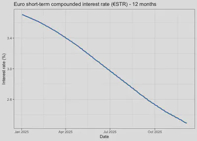
A new library: imfapi
A few months ago, someone in my LinkedIn network shared a post by Christopher Smith announcing the creation of a new library that “provides user-friendly functions for programmatic access to macroeconomic data from the ‘SDMX 3.0 IMF Data API’ of the International Monetary Fund.” The library in question is available on CRAN and works stably. Furthermore, it is part of the EconDataverse, which I recommend exploring. Below I will show, in a simplified way, how to access the same WEO data we saw earlier.
Using imfapi to extract WEO data
First, we load the library:
library(imfapi)
Then we retrieve the dataflows available in the IMF API:
dataflows <- imfapi::imf_get_dataflows()

dataflows |>
  dplyr::glimpse()
## Rows: 72
## Columns: 6
## $ id           <chr> "IMTS", "IL", "MFS_OFC", "ISORA_LATEST_DATA_PUB", "WPCPER…
## $ name         <chr> "International Trade in Goods (by partner country) (IMTS)…
## $ description  <chr> "The International trade in goods by partner country data…
## $ version      <chr> "1.0.0", "13.0.1", "7.0.0", "4.0.0", "6.0.0", "1.0.0", "9…
## $ agency       <chr> "IMF.STA", "IMF.STA", "IMF.STA", "ISORA", "IMF.STA", "IMF…
## $ last_updated <chr> "2025-03-28T17:18:44.429573Z", "2025-08-29T09:08:22.00741…
Now we filter for the WEO dataflow:
weo_flow <- dataflows |>
  dplyr::filter(id == "WEO")

weo_flow |>
  kableExtra::kable()
| id | name | description | version | agency | last_updated |
|---|---|---|---|---|---|
| WEO | World Economic Outlook (WEO) | The World Economic Outlook (WEO) database is created during the biannual WEO exercise, which begins in January and June of each year and results in the April and September/October WEO publication. Selected series from the publication are available in a database format. | 9.0.0 | IMF.RES | 2025-10-08T18:00:33.590181Z |
And we obtain the dimensions of the WEO dataflow:
dsd_weo <- imfapi::imf_get_datastructure(dataflow_id = "WEO")
dsd_weo |>
  kableExtra::kable()
| dimension_id | type | position |
|---|---|---|
| COUNTRY | Dimension | 0 |
| INDICATOR | Dimension | 1 |
| FREQUENCY | Dimension | 2 |
Next, we extract the codelists associated with the WEO dataflow:
dim_list <- list()

for (dim_id in dsd_weo$dimension_id) {
  dim_list[[dim_id]] <- imfapi::imf_get_codelists(
    dimension_ids = dim_id,
    dataflow_id   = "WEO"
  )
}

dim_list |>
  dplyr::bind_rows() |>
  dplyr::group_by(dimension_id) |>
  dplyr::summarise(n_codes = dplyr::n()) |>
  kableExtra::kable()
| dimension_id | n_codes |
|---|---|
| COUNTRY | 338 |
| FREQUENCY | 6 |
| INDICATOR | 145 |
In this case we have 338 codes for the COUNTRY dimension, 6 codes for the FREQUENCY dimension, and 145 valid codes for INDICATOR.
Finally, we extract WEO data for Bolivia and real GDP growth:
data <- imfapi::imf_get(
  dataflow_id = "WEO",
  dimensions  = list(
    COUNTRY   = "BOL",
    INDICATOR = "NGDP_RPCH",
    FREQUENCY = "A"
  )
)

data |>
  kableExtra::kable()
| COUNTRY | INDICATOR | FREQUENCY | TIME_PERIOD | OBS_VALUE |
|---|---|---|---|---|
| BOL | NGDP_RPCH | A | 1980 | 0.610 |
| BOL | NGDP_RPCH | A | 1981 | 0.300 |
| BOL | NGDP_RPCH | A | 1982 | -3.939 |
| BOL | NGDP_RPCH | A | 1983 | -4.042 |
| BOL | NGDP_RPCH | A | 1984 | -0.201 |
| BOL | NGDP_RPCH | A | 1985 | -1.676 |
| BOL | NGDP_RPCH | A | 1986 | -2.574 |
| BOL | NGDP_RPCH | A | 1987 | 2.463 |
| BOL | NGDP_RPCH | A | 1988 | 2.910 |
| BOL | NGDP_RPCH | A | 1989 | 3.790 |
| BOL | NGDP_RPCH | A | 1990 | 4.636 |
| BOL | NGDP_RPCH | A | 1991 | 5.267 |
| BOL | NGDP_RPCH | A | 1992 | 1.646 |
| BOL | NGDP_RPCH | A | 1993 | 4.269 |
| BOL | NGDP_RPCH | A | 1994 | 4.667 |
| BOL | NGDP_RPCH | A | 1995 | 4.678 |
| BOL | NGDP_RPCH | A | 1996 | 4.361 |
| BOL | NGDP_RPCH | A | 1997 | 4.954 |
| BOL | NGDP_RPCH | A | 1998 | 5.029 |
| BOL | NGDP_RPCH | A | 1999 | 0.427 |
| BOL | NGDP_RPCH | A | 2000 | 2.508 |
| BOL | NGDP_RPCH | A | 2001 | 1.684 |
| BOL | NGDP_RPCH | A | 2002 | 2.486 |
| BOL | NGDP_RPCH | A | 2003 | 2.711 |
| BOL | NGDP_RPCH | A | 2004 | 4.173 |
| BOL | NGDP_RPCH | A | 2005 | 4.421 |
| BOL | NGDP_RPCH | A | 2006 | 4.797 |
| BOL | NGDP_RPCH | A | 2007 | 4.564 |
| BOL | NGDP_RPCH | A | 2008 | 6.148 |
| BOL | NGDP_RPCH | A | 2009 | 3.357 |
| BOL | NGDP_RPCH | A | 2010 | 4.127 |
| BOL | NGDP_RPCH | A | 2011 | 5.204 |
| BOL | NGDP_RPCH | A | 2012 | 5.122 |
| BOL | NGDP_RPCH | A | 2013 | 6.796 |
| BOL | NGDP_RPCH | A | 2014 | 5.461 |
| BOL | NGDP_RPCH | A | 2015 | 4.857 |
| BOL | NGDP_RPCH | A | 2016 | 4.264 |
| BOL | NGDP_RPCH | A | 2017 | 4.195 |
| BOL | NGDP_RPCH | A | 2018 | 4.224 |
| BOL | NGDP_RPCH | A | 2019 | 2.217 |
| BOL | NGDP_RPCH | A | 2020 | -8.738 |
| BOL | NGDP_RPCH | A | 2021 | 6.111 |
| BOL | NGDP_RPCH | A | 2022 | 3.606 |
| BOL | NGDP_RPCH | A | 2023 | 3.082 |
| BOL | NGDP_RPCH | A | 2024 | 0.729 |
| BOL | NGDP_RPCH | A | 2025 | 0.600 |
In the table above we can see the WEO data for Bolivia and real GDP growth at annual frequency. The imfapi library considerably simplifies the data extraction process from the IMF API, allowing users to focus on data analysis rather than on the technical details of the SDMX API.
Conclusions
The aim of this post was to show that, for the applied analyst, working with SDMX APIs is not an end in itself but a way to build cleaner, more reproducible, and more scalable workflows. Instead of relying on manual downloads and poorly documented steps, SDMX allows us to find, understand, and extract macroeconomic data from different organizations under a common logic.
Through the IMF and ECB examples we saw that the general process—identifying the dataflow, reviewing its structure, consulting the codelists, and finally extracting the data—is repeated consistently, which makes it easier to automate and apply to other datasets. Moreover, tools like imfapi show how this approach can be simplified even further, reducing the technical burden so that most of the effort can be dedicated to analysis.
These two modifiers tell the server that we want the full structural information of the dataflow and all related elements—that is, the DSD, the concepts, and, crucially, all the codelists that depend on the dataflow. This saves us from having to manually search for which codelists exist, what they are called, or which version they are in. Instead, we obtain the complete WEO structure in a single, clean, and consistent call. ↩︎
For example, the
ESTdataflow, which corresponds to the euro short-term rate (€STR) and which we will investigate later, can be found here. ↩︎