Extracting Data from the IMF DataMapper API in R
In a previous post I showed how to access ECLAC data through its API. While this is quite useful, it is restricted to Latin American countries. In this post, therefore, I would like to extend data extraction to more general sources such as the International Monetary Fund (IMF).
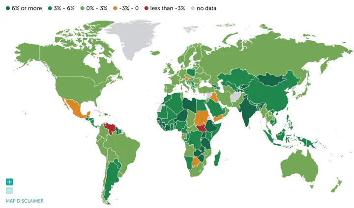
On the one hand, data can be extracted relatively directly from the DataMapper, which is quite general and contains information for most international analyses and comparisons one might wish to carry out, whether cross-sectional or panel. The API information is available here and is relatively easy to query. This will be our focus in this entry.
On the other hand, various international organizations have made their data available through a standard protocol, called SDMX, which allows access to data in a more or less homogeneous way. The IMF also provides an SDMX API, documented here. In this case, data extraction is a bit more complex, but there are R packages that make the task easier. In particular, the rsdmx package is quite useful for this purpose. However, its use will be explained in another post.
Data extraction from the IMF Data Mapper
For this case, the IMF provides the API through the following base URL https://www.imf.org/external/datamapper/api/v1/. From it, four main endpoints can be used to extract the data:
indicators: to obtain the list of available indicators.countries: to obtain the list of available countries.regions: to obtain the list of available regions.groups: to obtain the list of available country groups.
To understand the idea of an endpoint, simply paste the following URL into your preferred web browser https://www.imf.org/external/datamapper/api/v1/indicators. This will return plain text in JSON format with the list of available indicators:
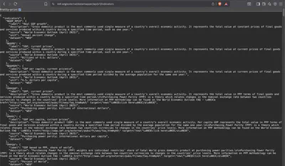
Therefore, the idea is to build a function that allows us to extract information from these endpoints in a more user-friendly format for data analysis and then filter the indicators or countries we are interested in.
A function to extract catalogs
First, we are going to use the jsonlite library (documentation here and here) which will allow us to extract information from the web.
The simplest way to do this is:
indicators <- jsonlite::fromJSON(txt='https://www.imf.org/external/datamapper/api/v1/indicators', simplifyVector = FALSE)

str(indicators, max.level = 2)
List of 2
 $ indicators:List of 133
  ..$ NGDP_RPCH         :List of 5
  ..$ NGDPD             :List of 5
  ..$ NGDPDPC           :List of 5
  ..$ PPPGDP            :List of 5
  ..$ PPPPC             :List of 5
  ..$ PPPSH             :List of 5
  ..$ PPPEX             :List of 5
  ..$ PCPIPCH           :List of 5
  ..$ PCPIEPCH          :List of 5
  ..$ LP                :List of 5
  ..$ BCA               :List of 5
  ..$ BCA_NGDPD         :List of 5
  ..$                   :List of 5
  ..$ LUR               :List of 5
  ..$ GGXCNL_NGDP       :List of 5
  ..$ GGXWDG_NGDP       :List of 5
  ..$ rev               :List of 5
  ..$ exp               :List of 5
  ..$ prim_exp          :List of 5
  ..$ ie                :List of 5
  ..$ pb                :List of 5
  ..$ d                 :List of 5
  ..$ rgc               :List of 5
  ..$ rltir             :List of 5
  ..$ extensive         :List of 5
  ..$ intensive         :List of 5
  ..$ total_theil       :List of 5
  ..$ SITC1_0           :List of 5
  ..$ SITC1_1           :List of 5
  ..$ SITC1_2           :List of 5
  ..$ SITC1_3           :List of 5
  ..$ SITC1_4           :List of 5
  ..$ SITC1_5           :List of 5
  ..$ SITC1_6           :List of 5
  ..$ SITC1_7           :List of 5
  ..$ SITC1_8           :List of 5
  ..$ SITC1_9           :List of 5
  ..$ SITC1_total       :List of 5
  ..$ DirectAbroad      :List of 5
  ..$ DirectIn          :List of 5
  ..$ PrivInexDI        :List of 5
  ..$ PrivInexDIGDP     :List of 5
  ..$ PrivOutexDI       :List of 5
  ..$ PrivOutexDIGDP    :List of 5
  ..$ Portfa            :List of 5
  ..$ Portfl            :List of 5
  ..$ EquityA           :List of 5
  ..$ EquityL           :List of 5
  ..$ DebtA             :List of 5
  ..$ DebtL             :List of 5
  ..$ OtherGov          :List of 5
  ..$ OtherA            :List of 5
  ..$ OtherL            :List of 5
  ..$ Deriv             :List of 5
  ..$ DebtForg          :List of 5
  ..$ GDP               :List of 5
  ..$ ka_new            :List of 5
  ..$ ka_in             :List of 5
  ..$ ka_out            :List of 5
  ..$ FM_ka             :List of 5
  ..$ Nonres_ka         :List of 5
  ..$ Res_ka            :List of 5
  ..$ Ka_eq             :List of 5
  ..$ Ka_bo             :List of 5
  ..$ Ka_mm             :List of 5
  ..$ Ka_ci             :List of 5
  ..$ Ka_dr             :List of 5
  ..$ Ka_cc             :List of 5
  ..$ Ka_fc             :List of 5
  ..$ Ka_gu             :List of 5
  ..$ Ka_di             :List of 5
  ..$ ka_ldi            :List of 5
  ..$ ka_ret            :List of 5
  ..$ ka_pct            :List of 5
  ..$ Reserves_ARA      :List of 5
  ..$ Reserves_M2       :List of 5
  ..$ Reserves_STD      :List of 5
  ..$ Reserves_M        :List of 5
  ..$ GRB_dummy         :List of 5
  ..$ GDI_TC            :List of 5
  ..$ GII_TC            :List of 5
  ..$ DEBT1             :List of 5
  ..$ Privatedebt_all   :List of 5
  ..$ HH_ALL            :List of 5
  ..$ NFC_ALL           :List of 5
  ..$ PVD_LS            :List of 5
  ..$ HH_LS             :List of 5
  ..$ NFC_LS            :List of 5
  ..$ PS_DEBT_GDP       :List of 5
  ..$ NFPS_DEBT_GDP     :List of 5
  ..$ GG_DEBT_GDP       :List of 5
  ..$ CG_DEBT_GDP       :List of 5
  ..$ GGXCNL_G01_GDP_PT :List of 5
  ..$ GGXONLB_G01_GDP_PT:List of 5
  ..$ GGCB_G01_PGDP_PT  :List of 5
  ..$ GGCBP_G01_PGDP_PT :List of 5
  ..$ GGR_G01_GDP_PT    :List of 5
  ..$ G_X_G01_GDP_PT    :List of 5
  ..$ G_XWDG_G01_GDP_PT :List of 5
  .. [list output truncated]
 $ api       :List of 2
  ..$ version      : chr "1"
  ..$ output-method: chr "json"
Which returns a list with indicators and other metadata, such as the name (label), its description (description), among others. To simplify the extraction logic, all steps are condensed into the get_catalog() function defined below:
get_catalog <- function(path,
                        base = "https://www.imf.org/external/datamapper/api/v1") {
  raw <- jsonlite::fromJSON(sprintf("%s/%s", base, path), simplifyVector = FALSE)

  # if raw[[path]] exists, use it; otherwise, use raw
  obj <- if (!is.null(raw[[path]])) raw[[path]] else raw

  obj$api <- NULL  # remove metadata

  tibble::tibble(
    code  = names(obj),
    label = vapply(obj, function(x) if (is.null(x$label)) NA_character_ else x$label,
                   character(1), USE.NAMES = FALSE)
  )
}
With this function we can extract catalogs of indicators, countries, regions, and groups of countries and organize them into a dataframe (or tibble) as follows:
indicators <- get_catalog("indicators")

head(indicators, 10)
# A tibble: 10 × 2
   code      label
   <chr>     <chr>
 1 NGDP_RPCH "Real GDP growth"
 2 NGDPD     "GDP, current prices"
 3 NGDPDPC   "GDP per capita, current prices\n"
 4 PPPGDP    "GDP, current prices"
 5 PPPPC     "GDP per capita, current prices"
 6 PPPSH     "GDP based on PPP, share of world"
 7 PPPEX     "Implied PPP conversion rate"
 8 PCPIPCH   "Inflation rate, average consumer prices"
 9 PCPIEPCH  "Inflation rate, end of period consumer prices"
10 LP        "Population"
We can do the same with countries, regions, and groups of countries, though reproducing with regions and groups is left to the reader:
countries <- get_catalog("countries")

head(countries, 10)
# A tibble: 10 × 2
   code  label
   <chr> <chr>
 1 ABW   Aruba
 2 AFG   Afghanistan
 3 AGO   Angola
 4 AIA   Anguilla
 5 ALB   Albania
 6 ARE   United Arab Emirates
 7 ARG   Argentina
 8 ARM   Armenia
 9 ASM   American Samoa
10 ATG   Antigua and Barbuda
Extracting specific data
Once we have the codes of the indicators and countries we are interested in, we can proceed to extract specific data. To do this, the IMF also shows us how to query the indicators. For example, if we wanted to extract real GDP growth (NGDP_RPCH) for Bolivia (BOL) between 2015 and 2020, we would query the following URL:https://www.imf.org/external/datamapper/api/v1/NGDP_RPCH/BOL?periods=2015,2016,2017,2018,2019,2020
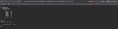
In R we could extract it as follows:
ngdp_bol <- jsonlite::fromJSON(txt='https://www.imf.org/external/datamapper/api/v1/NGDP_RPCH/BOL?periods=2015,2016,2017,2018,2019,2020', simplifyVector = FALSE)

ngdp_bol
$values
$values$NGDP_RPCH
$values$NGDP_RPCH$BOL
$values$NGDP_RPCH$BOL$`2015`
[1] 4.9

$values$NGDP_RPCH$BOL$`2016`
[1] 4.3

$values$NGDP_RPCH$BOL$`2017`
[1] 4.2

$values$NGDP_RPCH$BOL$`2018`
[1] 4.2

$values$NGDP_RPCH$BOL$`2019`
[1] 2.2

$values$NGDP_RPCH$BOL$`2020`
[1] -8.7


$api
$api$version
[1] "1"

$api$`output-method`
[1] "json"
If we wanted to extract information for several countries, such as Bolivia and the United States:
jsonlite::fromJSON(txt='https://www.imf.org/external/datamapper/api/v1/NGDP_RPCH/BOL/USA/?periods=2015,2016', simplifyVector = FALSE)
$values
$values$NGDP_RPCH
$values$NGDP_RPCH$BOL
$values$NGDP_RPCH$BOL$`2015`
[1] 4.9

$values$NGDP_RPCH$BOL$`2016`
[1] 4.3


$values$NGDP_RPCH$USA
$values$NGDP_RPCH$USA$`2015`
[1] 2.9

$values$NGDP_RPCH$USA$`2016`
[1] 1.8


$api
$api$version
[1] "1"

$api$`output-method`
[1] "json"
To condense everything in one place, we can define the following function get_data():
get_data <- function(indicators, areas, years = NULL,
                           base = "https://www.imf.org/external/datamapper/api/v1") {

  all_out <- vector("list", length(indicators))
  names(all_out) <- indicators

  for (j in seq_along(indicators)) {
    indicator <- indicators[j]

    # 1) Single call per indicator with multiple areas
    url <- sprintf("%s/%s/%s", base, indicator, paste(areas, collapse = "/"))
    x <- jsonlite::fromJSON(url, simplifyVector = FALSE)

    out_list <- vector("list", length(areas))
    names(out_list) <- areas

    for (i in seq_along(areas)) {
      area <- areas[i]
      node <- x$values[[indicator]][[area]]

      if (is.null(node)) {
        message("No data for indicator='", indicator, "' and area='", area, "'.")
        out_list[[i]] <- data.frame(code = character(), year = integer(), value = double(),
                                    indicator = character(), stringsAsFactors = FALSE)
        next
      }

      yrs_avail <- sort(as.integer(names(node)[grepl("^[0-9]{4}$", names(node))]))
      if (!length(yrs_avail)) {
        out_list[[i]] <- data.frame(code = character(), year = integer(), value = double(),
                                    indicator = character(), stringsAsFactors = FALSE)
        next
      }

      vals <- as.numeric(unlist(node[as.character(yrs_avail)], use.names = FALSE))
      df <- data.frame(code = area, year = yrs_avail, value = vals,
                       indicator = indicator, stringsAsFactors = FALSE)

      # Year trimming (if provided), with boundary warnings per country
      if (!is.null(years)) {
        yrs_req <- sort(unique(as.integer(years)))
        first_avail <- min(yrs_avail); last_avail <- max(yrs_avail)

        if (min(yrs_req) < first_avail)
          message("[", area, "][", indicator, "] No data returned from ",
                  min(yrs_req), " to ", first_avail - 1,
                  " (first available year: ", first_avail, ").")

        if (max(yrs_req) > last_avail)
          message("[", area, "][", indicator, "] No data returned from ",
                  last_avail + 1, " to ", max(yrs_req),
                  " (last available year: ", last_avail, ").")

        df <- df[df$year %in% yrs_req, , drop = FALSE]
      }

      out_list[[i]] <- df
    }

    all_out[[j]] <- do.call(rbind, out_list)
  }

  res <- do.call(rbind, all_out)
  rownames(res) <- NULL
  res
}
The get_data() function queries the IMF DataMapper API to download, in a single call, time series of an economic indicator (indicator) for one or multiple countries (areas), returning the results as a long-format data.frame with columns for country, year, value, and indicator. Internally, it extracts from the JSON the available years and values for each country, builds a data.frame per area, and, if the user specifies a range of years (years), trims the information to that range showing messages when requesting years outside those available. Finally, it combines all results into a single dataset ready for analysis or visualization.
For example, to extract real GDP growth (NGDP_RPCH) for Bolivia (BOL) and the United States (USA) between 2015 and 2020, we would do:
get_data(
  indicator = "NGDP_RPCH",
  area      = c("BOL","USA"),
  years     = 2010:2012
)
  code year value indicator
1  BOL 2010   4.1 NGDP_RPCH
2  BOL 2011   5.2 NGDP_RPCH
3  BOL 2012   5.1 NGDP_RPCH
4  USA 2010   2.7 NGDP_RPCH
5  USA 2011   1.6 NGDP_RPCH
6  USA 2012   2.3 NGDP_RPCH
A country snapshot
For example, once we have the information, we can analyze the situation of certain countries. Let’s illustrate with Bolivia.
First, load the required libraries:
library(tidyverse)
Then, from the indicators variable we created earlier, select the indicators of interest:
selected_ind <- c("NGDP_RPCH", # real GDP growth
                "LUR", # unemployment rate
                "PCPIPCH", # inflation
                "BCA_NGDPD", # current account as % of GDP
                "GGXCNL_NGDP", # general government fiscal balance as % of GDP
                "Reserves_M" # international reserves over imports
                )
Next, select the countries of interest:
areas <- c("BOL")
Finally, extract the data for the period 2010–2023:
data <- get_data(indicators = selected_ind,
                 areas      = areas,
                 years      = 2000:2025
                 )
data <- data |>
  left_join(indicators, by = c("indicator" = "code"))

data |>
  slice_sample(n = 10)
   code year value indicator                                   label
1   BOL 2022   3.6 NGDP_RPCH                         Real GDP growth
2   BOL 2025   1.1 NGDP_RPCH                         Real GDP growth
3   BOL 2011   5.2 NGDP_RPCH                         Real GDP growth
4   BOL 2009   3.3   PCPIPCH Inflation rate, average consumer prices
5   BOL 2001   8.5       LUR                       Unemployment rate
6   BOL 2007   7.7       LUR                       Unemployment rate
7   BOL 2011   9.9   PCPIPCH Inflation rate, average consumer prices
8   BOL 2023   3.1 NGDP_RPCH                         Real GDP growth
9   BOL 2021   3.9 BCA_NGDPD Current account balance, percent of GDP
10  BOL 2016   4.3 NGDP_RPCH                         Real GDP growth
Graphically:
data |>
  ggplot(aes(x = year, y = value, color = code)) +
  geom_line(size = 1.2, color ='steelblue') +
  geom_hline(yintercept = 0, linetype = "dashed", color = "red") +
  facet_wrap(~ label, scales = "free_y", ncol = 2) +
  labs(title = NULL,
       x = "Year",
       y = "Value",
       color = "Country") +
  theme_bw() +
  theme(legend.position = "none")

Or, for example, for the case of Spain:
selected_ind <- c("NGDP_RPCH", # real GDP growth
                "LUR", # unemployment rate
                "PCPIPCH", # inflation
                "BCA_NGDPD", # current account as % of GDP
                "GGXCNL_NGDP", # general government fiscal balance as % of GDP
                "GGCBP_G01_PGDP_PT" # public debt as % of GDP
                )

data_esp <- get_data(indicators = selected_ind,
                 areas      = 'ESP',
                 years      = 2000:2025
                 )
data_esp <- data_esp |>
  left_join(indicators, by = c("indicator" = "code"))

data_esp |>
  ggplot(aes(x = year, y = value, color = code)) +
  geom_line(size = 1.2, color ='steelblue') +
  geom_hline(yintercept = 0, linetype = "dashed", color = "red") +
  facet_wrap(~ label, scales = "free_y", ncol = 2) +
  labs(title = NULL,
       x = "Year",
       y = "Value",
       color = "Country") +
  theme_bw() +
  theme(legend.position = "none")

Conclusions
In this post we saw how to extract data from the IMF through its Data Mapper API. We defined two functions, get_catalog() and get_data(), which facilitate the extraction of indicator and country catalogs, as well as the retrieval of specific data for economic analysis. Finally, we illustrated how to use this data to perform a graphical analysis of economic indicators for countries such as Bolivia and Spain. This methodology enables efficient and structured access to international economic data, facilitating comparative analysis and informed decision-making.