Data Extraction from ECLAC in R and Application to Inflation in Bolivia

For the past few months, the Bolivian economic situation has been in constant deterioration: sustained fiscal deficit, depletion of international reserves, and the consequent breakdown of the fixed exchange rate, among others. One of the indicators where the problem has manifested is inflation which, as will be seen below, has been rising considerably.

However, when it first began to take off, some analysts argued that it was actually a transitory problem because non-tradable goods—those produced locally and without international competition, such as services or rents—were not increasing in price.

This led me to look for an available indicator to verify this claim and, fortunately, ECLAC already had some measures ready for analysis. What’s more, there is also an API through which, by entering the ID of the indicator to be analyzed, the data can be obtained automatically.

Therefore, the objective of this post is twofold: on the one hand, to show how data can be extracted from ECLAC, and on the other, as a practical case, to analyze the evolution of inflation in Bolivia and compare it with that of different countries in the region.

Extracting data from ECLAC

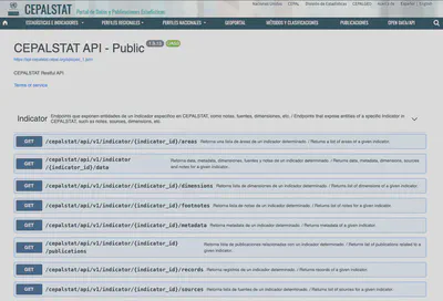
To extract data from ECLAC, you can use the API they make available. The API documentation is available at this link.

First, however, let’s load the libraries we will use in R:

library(tidyverse)
library(readxl)

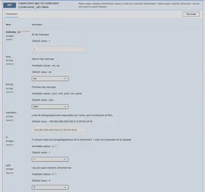
Now, as shown in the documentation, the URL to download the data is:
https://api-cepalstat.cepal.org/cepalstat/api/v1/indicator/{indicator_id}/data.
Here, the {indicator_id} part must be replaced with the ID of the indicator you want to analyze. In addition, different parameters can be specified, such as the language (lang) or the download format (format). These parameters are added at the end of the URL, separated by &. For example, to download the data in Excel format and in Spanish, you would add ?format=excel&lang=es at the end of the URL. The full list of parameters is available in the documentation:

How do we get the indicator_id? There are different ways to do this. The “manual” way would be browsing through CEPAL’s data visualizer, downloading the dataset as .xlsx, and then looking up the ID in the metadata tab.

A more automatic way is to download the full list of available indicators. This can also be done with a call to the API, but this time using the URL:
https://api-cepalstat.cepal.org/cepalstat/api/v1/thematic-tree.
Again, you can specify the format and lang parameters. For example, to download the full list of indicators in Spanish and in Excel format, you would use the URL:
https://api-cepalstat.cepal.org/cepalstat/api/v1/thematic-tree?format=excel&lang=es.

The following code shows how to download this list and load it into R:

tmp <- tempfile(fileext = ".xlsx")  
download.file(  
  "https://api-cepalstat.cepal.org/cepalstat/api/v1/thematic-tree?format=excel&lang=es",  
  destfile = tmp, mode = "wb"  
)  

indicators <- read_xlsx(tmp) |>   
  filter(type == "indicator") |>  
  select(id, name)  

indicators |>   
  glimpse()

Rows: 1,957  
Columns: 2  
$ id   <dbl> 4788, 4789, 4792, 4793, 4795, 4787, 4786, 3770, 4784, 4785, 4790,…  
$ name <chr> "Total population, by sex", "Population, by age groups, by sex",…

What does the code above do? First, it creates a temporary file to download the list of indicators. Then, it uses the download.file function to download the file from the specified URL and save it to the temporary file. After that, it uses the read_xlsx function from the readxl package to read the Excel file and load it into a data frame called indicators. Finally, it filters the rows to keep only those of type “indicator” and selects only the id and name columns. The glimpse function provides a quick view of the resulting data frame.

As you can see, there are 1,957 indicators available. For example, the indicator with ID 4788 corresponds to “Total population, by sex,” while the indicator with ID 4789 corresponds to “Population, by age groups, by sex,” and so on.

On this list, stored in the indicators data frame, you can run searches to find the indicators you are interested in.

In the case of price indices:

indicators |> 
  filter(str_detect(name, "Indice de precios"))

# A tibble: 7 × 2
     id name                                                
  <dbl> <chr>                                               
1  1684 Indice de precios al consumidor, alimentos y bebidas
2  4747 Indice de precios al consumidor resto               
3   365 Indice de precios al consumidor                     
4   764 Indice de precios al consumidor subyacente          
5   762 Indice de precios al consumidor en transables       
6   763 Indice de precios al consumidor en no transables    
7   544 Indice de precios al por mayor

Thus, the indicators of interest are mainly those with IDs 365, 762, 763, 764.

For example, to download the Consumer Price Index (CPI):

tmp <- tempfile(fileext = ".xlsx")
download.file(
  "https://api-cepalstat.cepal.org/cepalstat/api/v1/indicator/365/data?format=excel&in=1&lang=en",
  destfile = tmp, mode = "wb"
)

ipc <- read_xlsx(tmp) |> 
  janitor::clean_names()

ipc |> 
  glimpse()

Rows: 16,692
Columns: 8
$ indicator        <chr> "Consumer price index", "Consumer price index", "Cons…
$ years_estandar   <chr> "1980", "1980", "1980", "1980", "1980", "1980", "1980…
$ months           <chr> "January", "January", "January", "January", "January"…
$ country_estandar <chr> "Argentina", "Bolivia (Plurinational State of)", "Bra…
$ value            <dbl> 1.19815e-07, 1.40000e-04, 3.01600e-10, 7.32000e-01, 5…
$ unit             <chr> "Index", "Index", "Index", "Index", "Index", "Index",…
$ notes_ids        <chr> "2820", "3776,8658", "2824,5933", "2826,5935", "5938,…
$ source_id        <dbl> 256, 273, 258, 259, 262, 937, 277, 265, 925, 271, 256…

In this way we can download the data for different indicators and analyze them systematically.

Inflation in Bolivia

General inflation

Now, let’s see how inflation has behaved in Bolivia. For this, we use the CPI we just downloaded and calculate year-on-year inflation:

ipc_clean <- ipc |>
  mutate(Country = ifelse(grepl('Bolivia',country_estandar), 'Bolivia', country_estandar),
         Date_str = paste0(months, "-", years_estandar),
         Date = lubridate::my(Date_str),
         ) |>
  select(Date, Country, value) |> 
  arrange(Country, Date) |>
  group_by(Country) |>
  mutate(Inf_12m = (value/lag(value, 12) - 1) * 100) |>
  ungroup() |>
  filter(!is.na(Inf_12m))

Now, let’s plot year-on-year inflation in Bolivia:

ipc_clean |> 
  filter(Country == "Bolivia",
         Date >= as.Date("2018-01-01")
         ) |>
 ggplot(aes(x = Date)) +
  geom_line(aes(y = Inf_12m, color = "Inflation"), size = 1, color = 'red') +
  labs(title = "Year-on-year general inflation in Bolivia",
       x = NULL,
       y = "Inflation (%)",
       color = "",
              caption = "\nSource: Own elaboration based on ECLAC."
       ) +
  theme_bw(base_family = 'Latin Modern Roman') +
  scale_x_date(date_labels = "%b-%Y", date_breaks = "3 months",
               limits = as.Date(c("2018-01-01", "2025-08-01"))
               ) +
  theme(axis.text.x = element_text(angle = 90, vjust = 0.5),
        plot.caption = element_text(hjust = 0, face = "italic"),
        panel.grid.minor = element_blank(),
        legend.position = "none")

How does inflation in Bolivia compare with that of other countries in the region?

color <- "gray70"

ipc_clean |>
  filter(Country %in% c("Bolivia", "Paraguay", "Brazil", "Chile", "Colombia", 
                        "Mexico", "Peru", "Uruguay", "Ecuador", "Panama", 
                        "Costa Rica", "El Salvador"),
         Date >= as.Date("2018-01-01")) |>
  ggplot(aes(x = Date, y = Inf_12m, color = Country,
             alpha = ifelse(Country == "Bolivia", "Bolivia", "Other"))) +
  geom_line(size = 1) +
  labs(title = "Year-on-year inflation in Bolivia versus other countries in the region",
       x = NULL,
       y = "Inflation (%)",
       color = "",
       caption = "\nSource: Own elaboration based on INE.\nThe countries listed are: Paraguay, Brazil, Chile, Colombia, Mexico, Peru, Uruguay, Ecuador, Panama, Costa Rica and El Salvador.") +
  theme_bw(base_family = "Latin Modern Roman") +
  scale_x_date(date_labels = "%b-%Y", date_breaks = "3 months",
               limits = as.Date(c("2018-01-01", "2025-08-01"))) +
  scale_color_manual(values = c("Bolivia" = "red", 
                                "Paraguay" = color, "Brazil" = color,
                                "Chile" = color, "Colombia" = color,
                                "Mexico" = color, "Peru" = color,
                                "Uruguay" = color, "Ecuador" = color,
                                "Panama" = color, "Costa Rica" = color,
                                "El Salvador" = color)) +
  scale_alpha_manual(values = c("Bolivia" = 1, "Other" = 0.4), guide = "none") +
  theme(axis.text.x = element_text(angle = 90, vjust = 0.5),
        plot.caption = element_text(hjust = 0, face = "italic"),
        panel.grid.minor = element_blank(),
        legend.position = "none")

Core inflation

Another interesting indicator is core inflation, which excludes food and energy prices, as these tend to be more volatile. ECLAC also provides this indicator (ID 764).

tmp <- tempfile(fileext = ".xlsx")
download.file(
  "https://api-cepalstat.cepal.org/cepalstat/api/v1/indicator/764/data?format=excel&in=1&lang=en",
  destfile = tmp, mode = "wb"
)

ipc_core <- read_xlsx(tmp) |> 
  janitor::clean_names()

ipc_core |>
  glimpse()

Rows: 10,553
Columns: 8
$ indicator        <chr> "Core inflation", "Core inflation", "Core inflation",…
$ years_estandar   <chr> "1990", "1991", "1992", "1993", "1994", "1995", "1996…
$ months           <chr> "January", "January", "January", "January", "January"…
$ country_estandar <chr> "Argentina", "Argentina", "Argentina", "Argentina", "…
$ value            <dbl> 0.65900, 5.77200, 10.00600, 11.15600, 11.65100, 13.38…
$ unit             <chr> "Core Inflation", "Core Inflation", "Core Inflation",…
$ notes_ids        <chr> "2820,7747,7748", "2820,7747,7748", "2820,7747,7748",…
$ source_id        <dbl> 256, 256, 256, 256, 256, 256, 256, 256, 256, 256, 256…

Now, let’s clean the data and calculate year-on-year inflation:

ipc_core_clean <- ipc_core |>
  mutate(Country = ifelse(grepl('Bolivia',country_estandar), 'Bolivia', country_estandar),
         Date_str = paste0(months, "-", years_estandar),
         Date = lubridate::my(Date_str),
  ) |>
  select(Date, Country, value) |>
  arrange(Country, Date) |>
  group_by(Country) |>
  mutate(Inf_12m_core = (value/lag(value, 12) -
                          1) * 100) |>
  ungroup() |>
  filter(!is.na(Inf_12m_core))

Now, let’s plot core inflation in Bolivia:

ipc_core_clean |>
  filter(Country == "Bolivia",
         Date >= as.Date("2018-01-01")
  ) |>
  ggplot(aes(x = Date)) +
  geom_line(aes(y = Inf_12m_core, color = "Inflation"), color = "red", size = 1) +
  labs(title = "Year-on-year core inflation in Bolivia",
       x = NULL,
       y = "Inflation (%)",
       color = "",
       caption = "\nSource: Own elaboration based on ECLAC."
  ) +
  theme_bw(base_family = 'Latin Modern Roman') +
  scale_x_date(date_labels = "%b-%Y", date_breaks = "3 months"
               , limits = as.Date(c("2018-01-01", "2025-08-01"))
  ) +
  theme(axis.text.x = element_text(angle = 90, vjust = 0.5),
        plot.caption = element_text(hjust = 0, face = "italic"),
        panel.grid.minor = element_blank(),
        legend.position = "none")

How does core inflation in Bolivia compare with that of other countries in the region?

ipc_core_clean |>
  filter(Country %in% c("Bolivia", "Paraguay", "Brazil", "Chile", "Colombia",
                        "Peru", "Uruguay", "Ecuador", "Panama",
                        "Costa Rica", "El Salvador"),
         Date >= as.Date("2018-01-01")) |>
  ggplot(aes(x = Date, y = Inf_12m_core, color = Country,
             alpha = ifelse(Country == "Bolivia", "Bolivia", "Other"))) +
  geom_line(size = 1) +
  labs(title = "Year-on-year core inflation in Bolivia versus other countries in the region",
       x = NULL,
       y = "Inflation (%)",
       color = "",
       caption = "\nSource: Own elaboration based on ECLAC.\nThe countries listed are: Paraguay, Brazil, Chile, Colombia, Peru, Uruguay, Ecuador, Panama, Costa Rica and El Salvador.") +
  theme_bw(base_family = "Latin Modern Roman") +
  scale_x_date(date_labels = "%b-%Y", date_breaks = "3 months",
               limits = as.Date(c("2018-01-01", "2025-08-01"))) +
  scale_color_manual(values = c("Bolivia" = "red",
                                "Paraguay" = color, "Brazil" = color,
                                "Chile" = color, "Colombia" = color,
                                "Mexico" = color, "Peru" = color,
                                "Uruguay" = color, "Ecuador" = color,
                                "Panama" = color, "Costa Rica" = color,
                                "El Salvador" = color)) +
  scale_alpha_manual(values = c("Bolivia" = 1, "Other" = 0.4), guide = "none") +
  theme(axis.text.x = element_text(angle = 90, vjust = 0.5),
        plot.caption = element_text(hjust = 0, face = "italic"),
        panel.grid.minor = element_blank(),
        legend.position = "none")

Inflation of tradables and non-tradables

Finally, let’s look at the evolution of tradable and non-tradable goods prices. ECLAC also has these indicators available (IDs 762 and 763, respectively).

tmp <- tempfile(fileext = ".xlsx")
download.file(
  "https://api-cepalstat.cepal.org/cepalstat/api/v1/indicator/762/data?format=excel&in=1&lang=en",
  destfile = tmp, mode = "wb"
)

ipc_transable <- read_xlsx(tmp) |> 
  janitor::clean_names()

ipc_transable |>
  glimpse()

Rows: 10,753
Columns: 8
$ indicator        <chr> "Tradable consumer price index", "Tradable consumer p…
$ years_estandar   <chr> "1990", "1991", "1992", "1993", "1994", "1995", "1996…
$ months           <chr> "January", "January", "January", "January", "January"…
$ country_estandar <chr> "Argentina", "Argentina", "Argentina", "Argentina", "…
$ value            <dbl> 0.55000, 5.32400, 9.55800, 11.57400, 12.63700, 12.697…
$ unit             <chr> "Index of Transable goods", "Index of Transable goods…
$ notes_ids        <chr> "2820,7747,7748", "2820,7747,7748", "2820,7747,7748",…
$ source_id        <dbl> 256, 256, 256, 256, 256, 256, 256, 256, 256, 256, 256…

tmp <- tempfile(fileext = ".xlsx")
download.file(
  "https://api-cepalstat.cepal.org/cepalstat/api/v1/indicator/763/data?format=excel&in=1&lang=en",
  destfile = tmp, mode = "wb"
)

ipc_nontransable <- read_xlsx(tmp) |> 
  janitor::clean_names()
ipc_nontransable |>
  glimpse()

Rows: 10,755
Columns: 8
$ indicator        <chr> "Non-tradable consumer price index", "Non-tradable co…
$ years_estandar   <chr> "1990", "1991", "1992", "1993", "1994", "1995", "1996…
$ months           <chr> "January", "January", "January", "January", "January"…
$ country_estandar <chr> "Argentina", "Argentina", "Argentina", "Argentina", "…
$ value            <dbl> 0.57400, 5.61200, 9.48800, 11.03800, 11.91800, 12.732…
$ unit             <chr> "Index of non-tradable goods and services", "Index of…
$ notes_ids        <chr> "2820,7747,7748", "2820,7747,7748", "2820,7747,7748",…
$ source_id        <dbl> 256, 256, 256, 256, 256, 256, 256, 256, 256, 256, 256…

Now, let’s clean the data and calculate year-on-year inflation:

ipc_transable_clean <- ipc_transable |>
  mutate(Country = ifelse(grepl('Bolivia',country_estandar), 'Bolivia', country_estandar),
         Date_str = paste0(months, "-", years_estandar),
         Date = lubridate::my(Date_str),
  ) |>
  select(Date, Country, value) |>
  arrange(Country, Date) |>
  group_by(Country) |>
  mutate(Inf_12m_transable = (value/lag(value, 12) -1) * 100) |>
  ungroup() |>
  filter(!is.na(Inf_12m_transable))

ipc_nontransable_clean <- ipc_nontransable |>
  mutate(Country = ifelse(grepl('Bolivia',country_estandar), 'Bolivia', country_estandar),
         Date_str = paste0(months, "-", years_estandar),
         Date = lubridate::my(Date_str),
  ) |>
  select(Date, Country, value) |>
  arrange(Country, Date) |>
  group_by(Country) |>
  mutate(Inf_12m_nontransable = (value/lag(value, 12)-1) * 100) |>
  ungroup() |>
  filter(!is.na(Inf_12m_nontransable))
  
ipc_both <- ipc_transable_clean |>
  select(Date, Country, Inf_12m_transable) |>
  left_join(ipc_nontransable_clean |>
              select(Date, Country, Inf_12m_nontransable),
            by = c("Date", "Country"))

Now, let’s plot the inflation of tradable and non-tradable goods in Bolivia:

ipc_both |>
  filter(Country == "Bolivia",
         Date >= as.Date("2018-01-01")
  ) |>
  pivot_longer(cols = c(Inf_12m_transable, Inf_12m_nontransable),
               names_to = "Type", values_to = "Inflation") |>
  mutate(Type = recode(Type,
                       Inf_12m_transable = "Tradable goods",
                       Inf_12m_nontransable = "Non-tradable goods")) |>
  ggplot(aes(x = Date, y = Inflation, color = Type)) +
  geom_line(size = 1) +
  scale_color_manual(values = c("Tradable goods" = "gray80", "Non-tradable goods" = "red")) +
  labs(title = "Year-on-year inflation in Bolivia: tradable and non-tradable goods",
       x = NULL,
       y = "Inflation (%)",
       color = "",
       caption = "\nSource: Own elaboration based on ECLAC."
  ) +
  theme_bw(base_family = 'Latin Modern Roman') +
  scale_x_date(date_labels = "%b-%Y", date_breaks = "3 months" , limits = as.Date(c("2018-01-01", "2025-08-01"))
  ) +
  theme(axis.text.x = element_text(angle = 90, vjust = 0.5),
        plot.caption = element_text(hjust = 0, face = "italic"),
        panel.grid.minor = element_blank(),
        legend.position = "bottom")

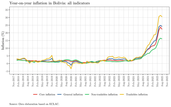
All inflations together

Finally, let’s look at all the inflation measures together:

ipc_clean |>
  filter(Country == "Bolivia",
         Date >= as.Date("2018-01-01")
  ) |>
  select(Date, Inf_12m) |>
  left_join(ipc_core_clean |>
              filter(Country == "Bolivia") |>
              select(Date, Inf_12m_core),
            by = "Date") |>
  left_join(ipc_both |>
              filter(Country == "Bolivia") |>
              select(Date, Inf_12m_transable, Inf_12m_nontransable),
            by = "Date") |>
  pivot_longer(cols = c(Inf_12m, Inf_12m_core, Inf_12m_transable, Inf_12m_nontransable),
               names_to = "Type", values_to = "Inflation") |>
  mutate(Type = recode(Type,
                       Inf_12m = "General inflation",
                       Inf_12m_core = "Core inflation",
                       Inf_12m_transable = "Tradables inflation",
                       Inf_12m_nontransable = "Non-tradables inflation")) |>
  ggplot(aes(x = Date, y = Inflation, color = Type)) +
  geom_line(size = 1, alpha = 1) +
  scale_color_manual(values = c("General inflation" = "#4682B4",
                                "Core inflation" = "#E74C3C",
                                "Tradables inflation" = "#F1C40F",
                                "Non-tradables inflation" = "#2ECC71")) +
  labs(title = "Year-on-year inflation in Bolivia: all indicators",
       x = NULL,
       y = "Inflation (%)",
       color = "",
       caption = "\nSource: Own elaboration based on ECLAC.") +
  theme_bw(base_family = 'Latin Modern Roman') +
  scale_x_date(date_labels = "%b-%Y", date_breaks = "3 months" , limits = as.Date(c("2018-01-01", "2025-08-01"))
  ) +
  scale_y_continuous(limits = c(-5, 35), breaks = seq(-5,35,5)  ) +
  theme(axis.text.x = element_text(angle = 90, vjust = 0.5),
        plot.caption = element_text(hjust = 0, face = "italic"),
        panel.grid.minor = element_blank(),
        legend.position = "bottom")

Thus, it can be observed that by August 2025 inflation ranged from 16.05% in the case of non-tradable goods to 30.43% for tradable goods.

Conclusions

This post showed how to extract data from ECLAC using its API and, as a practical case, analyzed the evolution of inflation in Bolivia and its comparison with other countries in the region. It was observed that inflation in Bolivia has been significantly higher than in other countries in the region, and that both tradable and non-tradable goods have experienced price increases, although non-tradables took a little longer to rise.